Modelos para Contagens e Proporções
Desenho Experimental e Análise Avançada de Dados Ecológicos
2025-11-25
Binomial Test
To test if the proportion of a given level of a nominal variable, differs from a hypothesized proportion (e.g., π = 0.5; π = 50%) we can resort to a binomial test
The test relies on the binomial distribution (a discrete distribution) and is pretty straightforward for directional (unilateral) tests or for when π = 50%
Binomial Test
The mathematically-inclined will find the Wikipedia pretty illuminating
Playing around with the binomial distribution in JASP’s “Distributions” model should be illuminating for all
Binomial Test
Test if the ratio of males/females differs from 50% in penguins:
Binomial Test
Test if the ratio of females/males differs across species:
    Exact binomial test

data:  counts
number of successes = 165, number of trials = 333, p-value = 0.9127
alternative hypothesis: true probability of success is not equal to 0.5
95 percent confidence interval:
 0.4405416 0.5505302
sample estimates:
probability of success
0.4954955 - No evidence that the ratio of females and males differs from 50%
Chi-Square Test for Counts
\(\chi^2 = \sum\limits_{r = 1}^r \sum\limits_{c = 1}^c \frac{(O_{(r,c)} - E_{(r,c)})^2}{E_{(r, c)}}\)
Observed frequency: The count in that cell
Expected frequency: \(E(row, column) = \frac{total_{row} \times total_{column}}{total_{table}}\)
Degrees of freedom (df): \(df = (r - 1) \times (c - 1); r/c = \text{number of rows/columns}\)
Chi-Square Test for Counts
Assumptions:
Independent counts
All (100%) expected counts must be equal or greater than one
80% of expected counts must be five or greater
Note: at least one variable should be nominal, or there are more suitable tests to perform
Chi-Square Test for Counts
Perform test:
Chi-Square Test for Counts
See results:
Chi-Square Test for Counts
Check assumptions:
Understanding the Results
           Adelie Chinstrap   Gentoo
  female 72.34234  33.69369 58.96396
  male   73.65766  34.30631 60.03604
         Adelie Chinstrap Gentoo
  female     73        34     58
  male       73        34     61
The more the observed counts differ from the expected counts the more evidence there is against the independence hypothesis (H0)
In this case there’s very little evidence of the variables being associated
Understanding the Results
              Adelie   Chinstrap      Gentoo
  female  0.14526881  0.08328145 -0.22047034
  male   -0.14526881 -0.08328145  0.22047034
The larger the difference between observed and expected the larger in absolute value the standard residuals will be.
Note these are z values, with no correction we would take |z| = 1.96 as significant evidence of difference (if we don’t correct for multiple comparisons)
Some Tests Are the Same
- Link (in case slide breaks)
Non-quantitative DVs
With a binomial DV we should fit a generalized linear model, or a generalized linear mixed model, of the binomial family
-
With the DV refers to count data we should fit a generalized linear model, or a generalized linear mixed model, of the poisson family
- Not required, but valued, for the individual assignment
Non-quantitative DVs
- With ordinal DVs we should fit a multinomial regression
- For models with only one IV, we can also perform a Spearman’s correlation test
- We can also pretend we can treat the IV as quantitativu
- Not expected for the individual assignment
Binomial Logistic Regression
Log-Odds
Probability: \(P = \frac{N_{favorable}}{N_{possible}}\)
Odds: \(O = \frac{P}{1 - P}\)
Log-odds/Logit (natural logarithm of odds): \(\ln(O) = \ln(\frac{P}{1 - P})\)
Example
Let’s predict if a passenger survived the tinatic:
library(car)
library(emmeans)

# Change default contrasts for categorical variables
options(contrasts = c("contr.sum", "contr.poly"))

# Import Data
ds <- read.csv("../../data/titanic.csv")
# Data Wrangling
# Ensure class is treated as qualitative
ds$Pclass <- paste0("class", ds$Pclass)
# Fit the model
model <- glm(Survived ~ Pclass * Sex, ds, family = "binomial")
# ANOVA table
results <- Anova(model, type = 3)
Exercise
- Look at the estimated marginal means and pairwise comparisons, but use
type = "response"in theemmeans()function call
Solutions
library(car)
library(emmeans)
library(ggplot2)

# Change default contrasts for categorical variables
options(contrasts = c("contr.sum", "contr.poly"))

# Import Data
ds <- read.csv("../../data/titanic.csv")
# Data Wrangling
# Ensure class is treated as qualitative
ds$Pclass <- paste0("class", ds$Pclass)
# Fit the model
model <- glm(Survived ~ Pclass * Sex, ds, family = "binomial")
# ANOVA Table (type III sums of squares)
results <- Anova(model, type = 3)
# Estimated Marginal Means
emm_pclass <- emmeans(model, ~ Pclass, type = "response")
emm_sex <- emmeans(model, ~ Sex, type = "response")
emm_int <- data.frame(emmeans(model, ~ Pclass * Sex, type = "response"))
# Multiple Comparisons
pc_pclass <- pairs(emm_pclass)
pc_pclass_sex <- pairs(emmeans(model, ~ Pclass | Sex, type = "response"))
pc_sex_pclass <- pairs(emmeans(model, ~ Sex | Pclass, type = "response"))
# Interaction Plots
# Note: y = prob NOT y = emmean;
#       ymin/max = asymp.L/UCL NOT ymin/max = lower/upper.CL
g_pclass_sex <- ggplot(emm_int, aes(x = Pclass, y = prob, color = Sex)) +
                geom_point() +
                geom_errorbar(aes(ymin = asymp.LCL, ymax = asymp.UCL)) +
                geom_line(aes(group = Sex)) +
                theme_classic()
# Species by target
g_sex_pclass <- ggplot(emm_int, aes(x = Sex, y = prob, color = Pclass)) +
                geom_point() +
                geom_errorbar(aes(ymin = asymp.LCL, ymax = asymp.UCL)) +
                geom_line(aes(group = Pclass)) +
                theme_classic()
Solutions
Solutions
Solutions
Solutions
 contrast        odds.ratio   SE  df null z.ratio p.value
 class1 / class2       2.98 1.20 Inf    1   2.713  0.0183
 class1 / class3      10.89 3.68 Inf    1   7.066 <0.0001
 class2 / class3       3.66 1.05 Inf    1   4.515 <0.0001

Results are averaged over the levels of: Sex
P value adjustment: tukey method for comparing a family of 3 estimates
Tests are performed on the log odds ratio scale
Solutions
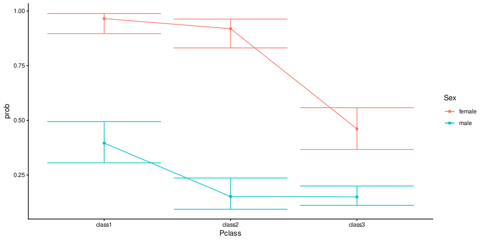
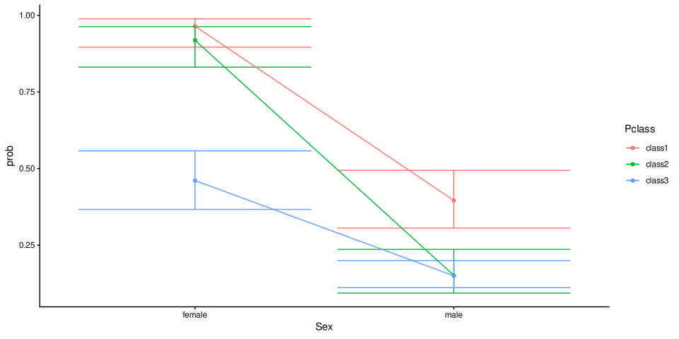
  Pclass    Sex      prob         SE  df  asymp.LCL asymp.UCL
1 class1 female 0.9647059 0.02000280 Inf 0.89629008 0.9885647
2 class2 female 0.9189189 0.03173090 Inf 0.83104363 0.9631181
3 class3 female 0.4607843 0.04935487 Inf 0.36667319 0.5577769
4 class1   male 0.3960396 0.04866457 Inf 0.30560310 0.4941922
5 class2   male 0.1515152 0.03603566 Inf 0.09345538 0.2362451
6 class3   male 0.1501976 0.02246106 Inf 0.11125800 0.1997035
Solutions
Solutions
Sex = female:
 contrast        odds.ratio     SE  df null z.ratio p.value
 class1 / class2       2.41  1.750 Inf    1   1.213  0.4453
 class1 / class3      31.99 19.800 Inf    1   5.588 <0.0001
 class2 / class3      13.26  6.230 Inf    1   5.501 <0.0001

Sex = male:
 contrast        odds.ratio     SE  df null z.ratio p.value
 class1 / class2       3.67  1.270 Inf    1   3.756  0.0005
 class1 / class3       3.71  0.998 Inf    1   4.874 <0.0001
 class2 / class3       1.01  0.334 Inf    1   0.031  0.9995

P value adjustment: tukey method for comparing a family of 3 estimates
Tests are performed on the log odds ratio scale - For women, only the third class differed from the first and second. For men, the first class differs from the second and third, but the second and third don’t differ.
Solutions
Solutions
Pclass = class1:
 contrast      odds.ratio    SE  df null z.ratio p.value
 female / male      41.68 25.90 Inf    1   6.000 <0.0001

Pclass = class2:
 contrast      odds.ratio    SE  df null z.ratio p.value
 female / male      63.47 32.40 Inf    1   8.141 <0.0001

Pclass = class3:
 contrast      odds.ratio    SE  df null z.ratio p.value
 female / male       4.83  1.28 Inf    1   5.938 <0.0001

Tests are performed on the log odds ratio scale - Regardless of which class they boarded, women are always more likely to survive than men, but the difference seems lower for the third class