Pressupostos dos Modelos/testes

Desenho Experimental e Análise Avançada de Dados Ecológicos

João O. Santos

joao.santos@ispa.pt

ISPA

2025-11-18

Assumptions

• I’ve (purposely) postponing mentioning model assumptions

• Given we followed the model comparison approach (Judd et al. 2017), it makes sense to discuss model assumptions towards the end, once we understand the basics of building statistical models

• Now it is finally time to understand model assumptions: what are they? what happens when they are violated? what can we do to address violations?

Theoretical Assumptions

• Many assumptions can be empirically assessed, but some are theoretical

• Generally speaking, the model should be properly specified to meet all the theoretical assumptions

Quantitative Dependent Variable

• The dependent variable is quantitative

Independence and/or Dependence

• Independent samples models: The independent variable/s define independent samples (for non-repeated measures models)

• Repeated measures models: the independent variable/s define/s repeated measures (for repeated measures ANOVA or linear mixed models)

• Mixed designs: one/some IV/s define independent samples and another/others repeated measures (split-plot/mixed ANOVAs or linear mixed models)

Empirically Testable Assumptions

• The relationship between the dependent and independent variables is linear (for quantitative variables)

Linearity

• For quantitative variables

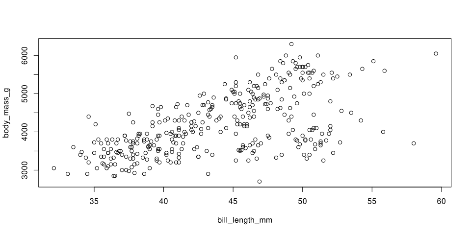
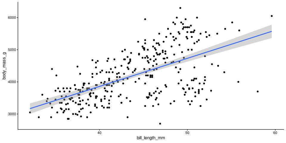
• Inspected by looking at scatterplots of DV ~ IV

• Only applicable for categorical predictors if there are interaction not featured in the model

Example

library(palmerpenguins)

ds <- penguins

model <- lm(body_mass_g ~ bill_length_mm, ds)

Linearity

With quick and dirty base R graph:

plot(body_mass_g ~ bill_length_mm, ds)

Linearity

With pretty ggplot2 graph:

library(ggplot2)

g <- ggplot(ds, aes(x = bill_length_mm, y = body_mass_g)) +
     geom_point() + geom_smooth(method = "lm") +
     theme_classic()

Linearity

With pretty ggplot2 graph:

print(g)

Linearity

Ways to address violations:

• Log transform the DV and IV

• Compute the square root of the DV and IVs

• Note: transforming the data means H0 and H1 will refer to the transformed data

Linearity

Ways to address violations:

• Fit a generalized linear model with an appropriate link function:
  • preferred if data follows a known non-linear pattern (e.g., exponential)
• Fit a non-parametric model

Normally Distributed Errors

• The errors (residuals) of the model follow the normal distribution:
  • \(\epsilon \sim N(0, \sigma)\)
• For categorical predictors it can also be said the dependent variable is normally distributed across all values of the independent variable/s

Normally Distributed Errors

• Shapiro-Wilk’s test:

  • Very sensitive, specially if N > 50

• Kolmogorov-Smirnov’s test with Lilliefors correction:

  • Less sensitive than SW, specially if N > 50

• Visual inspection of the histogram or density graph of the standardized residuals

• Visual inspection of the qq-plot of standardized residuals

  • preferred option

Getting Model Errors

# Store errors in a variable for an easier time working with them
errors <- resid(model)

Shapiro-Wilk

In base R:

shapiro.test(errors)

    Shapiro-Wilk normality test

data:  errors
W = 0.99144, p-value = 0.04502

length(errors)

[1] 342

• Significant evidence of non-normality (for α = .050), yet p is close to α (p = .045), and the test is too sensitive for this N

Shapiro-Wilk

With the performance package:

library(performance)

# Works with the model object/variable
check_normality(model)

Warning: Non-normality of residuals detected (p = 0.045).

Kormogorov-Smirnov With Lillifors

library(nortest)

lillie.test(errors)

    Lilliefors (Kolmogorov-Smirnov) normality test

data:  errors
D = 0.040585, p-value = 0.1859

• Not available in base R, requires nortest

• There is no significant evidence of non-normality (for α = .050)

Scale Residuals

• Working with scaled residuals (z scores) means we know they’ll have a mean of zero and standard deviation of one

• This means we can easily scale the graphs to range from minus three to plus three (M +/- 3 x SD) or some other multiple of the SD

Scale Residuals

# Transform errors into a data.frame with scaled residuals
errors <- data.frame(scaled_errors = scale(errors))

• Saving the errors in a data.frame will make them easier to work with in ggplot2

Histogram

In base R:

hist(errors$scaled_errors)

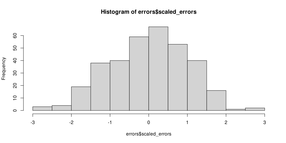
• Data looks mostly normal, but the graph isn’t the prettiest

Density Graph

With ggplot2:

# `dnorm` gives the density for the normal distribution
# `color = "red"` makes the line for the normal distribution red
g <- ggplot(errors, aes(x = scaled_errors)) +
     geom_density() + stat_function(fun = dnorm, color = "red") +
     theme_classic()

Density Graph

print(g)

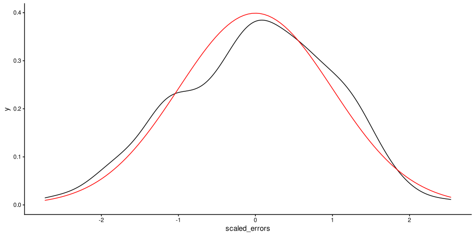
• Only small deviations from normality are seen on the graph

Q-Q Plot

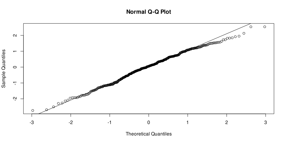
In base R:

# Q-Q plot
qqnorm(errors$scaled_errors)
# Add line
qqline(errors$scaled_errors)

Q-Q Plot

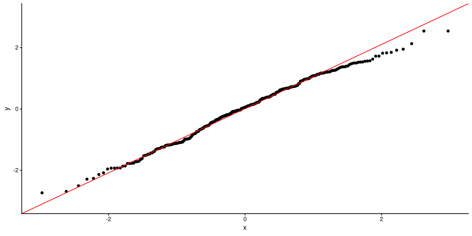
With ggplot2:

g <- ggplot(errors, aes(sample = scaled_errors)) +
     stat_qq() + stat_qq_line(color = "red") +
     theme_classic()

Q-Q Plot

print(g)

Q-Q Plot

Interpretation:

• I reckon it’s mostly normal, with slight deviations in the extreme ends of the tails

• Note: graphical inspection is subjective, just be consistent

Normally Distributed Errors

Ways to address violations:

• Log transform the DV, and/or IVs:

  • Useful if data is positively skewed

• Compute the square root of the DV and/or IVs

• Box-cox transform the DV

• Note: transforming the data means H0 and H1 will refer to the transformed data

Normally Distributed Errors

Ways to address violations:

• Fit a non-linear model:

  • preferred if the violation speaks of a specific non-linear relation (e.g., exponential)

• Fit a non-parametric model (these have different H0 and H1)

• Report it, and do nothing (specially when N is large)?

Homoscedasticity

\(\sigma_1^2 = \sigma_2^2 = \sigma_{\cdots} = \sigma_i^2\)

• Independent samples models: The variance of the DV is the same in all combinations of the levels of the IV/s

• Mixed designs: The variances of the DV is the same in all combinations of the levels of the between-units IV/s for all levels of the repeated measures IV/s

• Models with only repeated measures IV/s: only applicable to linear mixed models, repeated measures ANOVAs do not have that assumption (they assume sphericity, see next slides)

Homoscedasticity

Tested/inspected with:

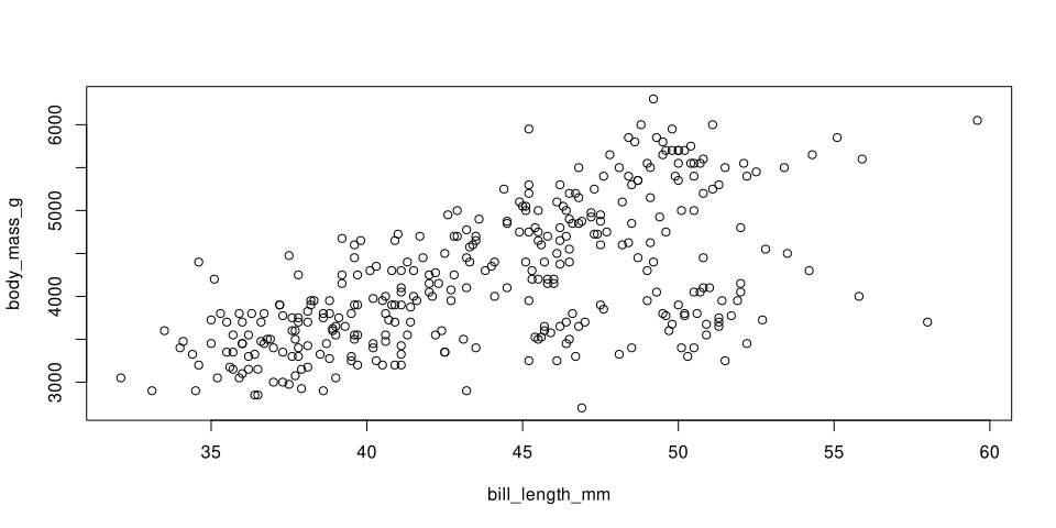
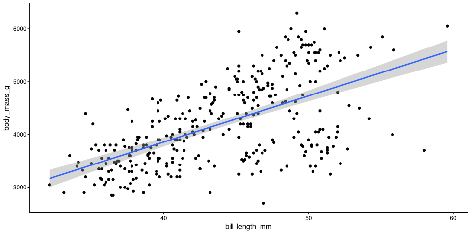
• A scatter plot of DV ~ IV (looking for similar dispersion along the graph, i.e., no funnels)
  • Useful for models with only one IV
• A scatter plot of predictions and residuals (looking for homogenous pattern, with no funnels)
  • Or the square root of residuals and predictions (looking for a flat line)
• Levene’s test:
  • Only applicable for categorical predictors
  • Formally called Brown-Forsythe test if based on the median

DV ~ IV Scatter Plot

In base R:

plot(body_mass_g ~ bill_length_mm, ds)

DV ~ IV Scatter Plot

With ggplot2:

g <- ggplot(ds, aes(x = bill_length_mm, y = body_mass_g)) +
     geom_point() + geom_smooth(method = "lm") +
     theme_classic()

DV ~ IV Scatter Plot

With ggplot2:

print(g)

DV ~ IV Scatter Plot

Interpretation (in regard to homo/heteroscedasticity):

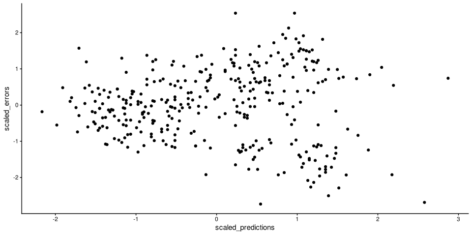
• We see a funneling pattern, with our model showing a better fit when predicting lower values for the DV, than when predicting higher values

• We make more errors predicting heavier body masses

• There is more variability in higher body masses when given as a function of bill length

Predictions ~ Errors

Get predictions:

# errors already has a column with the scaled residuals
# Let's add a column with the scaled predictions
errors$scaled_predictions <- scale(predict(model))

Predictions ~ Errors

g <- ggplot(errors, aes(x = scaled_predictions, y = scaled_errors)) +
     geom_point() + theme_classic()

print(g)

Predictions ~ Errors

Interpretation:

• Same as before

• We make more errors predicting heavier body masses

• There is more variability in higher body masses when given as a

Levene’s Test

• Levene’s test only works for categorical IV/s

• Let’s fit a One-Way ANOVA testing for differences in body mass between species

Levene’s Test

model <- lm(body_mass_g ~ species, ds)

Levene’s Test

Using the car package:

library(car)

leveneTest(model)

	Df	F value	Pr(>F)
group	2	5.120251	0.0064451
	339	NA	NA

Homoscedasticity

Ways to address violations:

• Fit a robust model

• Correct the test statistic (with categorical predictors one can apply the Welch or Brown-Forsythe correction)

Homoscedasticity

Ways to address violations:

• Fit a non-parametric model:
  • Namely, the Kruskal-Wallis test if there is only one IV
    • It tests for a different H0 and H1
    • It tests if the DV has a different distribution in different levels of the iV
    • A violation of homoscedasticity, already suggests the distributions differ across levels in their variances

Robust One-Way ANOVA

library(WRS2)

t1way(body_mass_g ~ species, ds)

Call:
t1way(formula = body_mass_g ~ species, data = ds)

Test statistic: F = 247.5234 
Degrees of freedom 1: 2 
Degrees of freedom 2: 118.49 
p-value: 0 

Explanatory measure of effect size: 0.91 
Bootstrap CI: [0.86; 0.97]

Sphericity

\(\sigma_{A-B}^2 = \sigma_{A-C}^2 = \sigma_{B-C}^2\)

• The variance of the differences between each measurement of the DV (e.g., A, B, C) is the same:

• Only applicable when (at least one of) the repeated measures IV/s has k > 2

• Only applicable to repeated measures ANOVAs or split-plot ANOVAs (i.e., not applicable to mixed models)

Sphericity

Ways to test/probe for violations:

• Looking at the value of Epsilon (ε < 0.7 suggests a violation)

• With Mauchly’s test of sphericity

Sphericity

Ways to address violations:

• Apply Greenhouse-Geisser, Huynd-Feldt, or Lower-Bound correction

• Fit a linear mixed model (mixed())

• Fit a robust model

• Note: afex automatically performs Mauchly’s tests (when applicable) and automatically applies the Greenhouse-Geisser correction

Sphericity

library(afex)

options(contrasts = c("contr.sum", "contr.poly"))
afex_options(es_aov = "pes")

ds <- read.csv("../../data/bryozoan_wrangled.csv")
ds <- subset(ds, Stage != "LARVAE")
model <- aov_4(Log10MR ~ Stage * Species + (Stage | Id), ds)

Sphericity

print(model)

Anova Table (Type 3 tests)

Response: Log10MR
         Effect     df  MSE          F  pes p.value
1       Species 1, 253 0.03 288.52 *** .533   <.001
2         Stage 1, 253 0.02 757.70 *** .750   <.001
3 Species:Stage 1, 253 0.02  16.84 *** .062   <.001
---
Signif. codes:  0 '***' 0.001 '**' 0.01 '*' 0.05 '+' 0.1 ' ' 1

• If afex::aov_4() or afex::aov_car() do not report a violation of sphericity it means Mauchly’s test of sphericity yields no significant evidence (for α = .05) for a violation.

Sphericity

# We can double-check with check_sphericity() if we want.
check_sphericity(model)

OK: Data seems to be spherical (p > .999).

• There is no evidence of sphericity being violated

Uncorrelated Predictors/IVs

• The independent variables are independent of one another (i.e., they are not correlated):

  • Also referred to as the absence of multicollinearity
  • Only applicable when there is more than one IV/predictor

• Inspected by looking at a correlation matrix with all IVs

• Inspected by looking at scatter plots of each IV as a function of another

• Inspected by looking at VIF and/or Tolerance:

  • Preferred, specially for more than 2 IVs

Uncorrelated Predictors/IVs

Fitting a multiple linear regression (quantitative IVs):

library(palmerpenguins)
library(performance)

# Load penguins data into `ds`
ds <- penguins

# Only main effects (no interactions) model for simplicity of example
model <- lm(body_mass_g ~ bill_length_mm + bill_depth_mm + flipper_length_mm, ds)

Uncorrelated Predictors/IVs

check_collinearity(model)

Term	VIF	VIF_CI_low	VIF_CI_high	SE_factor	Tolerance	Tolerance_CI_low	Tolerance_CI_high
bill_length_mm	1.865090	1.623085	2.201090	1.365683	0.5361671	0.4543202	0.6161108
bill_depth_mm	1.611292	1.418853	1.892145	1.269367	0.6206201	0.5285008	0.7047946
flipper_length_mm	2.673338	2.277269	3.192223	1.635034	0.3740642	0.3132613	0.4391224

Independently Distributed Errors

• The errors (residuals) are not autocorrelated (we cannot predict an error based on the error for the previous observation)

• More discussed/explored in regards to time-series models

• Tested with the Durbin-watson test

Independently Distributed Errors

library(performance)

check_autocorrelation(model)

OK: Residuals appear to be independent and not autocorrelated (p = 0.832).

Absence of Outliers

• Not necessarily a formal assumption, but the OLS estimator is very sensitive to them

• Different criteria are debated/recommended in the literature:

  • No standardized residual (zscore) or robust zscore larger than 3.291 (\(|z| < 3.291\))
  • No residual with a Cook’s distance greater than \(\frac{4}{n}\)
  • Boxplots with no value outside the inner barriers (usually: \(Q1 - (1.5 \times IQR); Q3 + (1.5 \times IQR)\))

Absence of Outliers

• Visual exploration of scatter, residual, and/or Q-Q plots

• For a great discussion and tutorial see Lüdecke et al

Absence of Outliers

library(performance)

check_outliers(model)

OK: No outliers detected.
- Based on the following method and threshold: cook (0.841).
- For variable: (Whole model)

• Don’t forget to read Lüdecke et al

Absence Outliers

Ways to address outliers:

• Pre-register an objective cutoff according to some metric/s to spot residuals

  • Remove outliers, and refit the model
  • Repeat until no outliers are found

• Fit a model on the entire dataset, and fit a model with the outliers removed, then check if the pattern of results holds

• Fit a model that’s robust against outliers (e.g., robustbase::lmrob(), robustlmm:rlmer())

Assumption Tests

Like other statistical tests, assumption tests have limitations:

• Power (the ability to detect an effect if there is one) increases with sample size

• For small sample sizes they often underestimate violations, and for large sample sizes they often overestimate (or flag small violations of little import)

• Thus, visual inspection is often recommended (e.g., Judd et al 2017)

Assumption Tests

• Note: model estimates and statistical test are not equally affected by all violations, but that is a complex debate (see Hu & Plonski 2019; Knief & Forstmeier 2021; Schielzeth et al 2020; Nimon 2012; Osborne 2013)

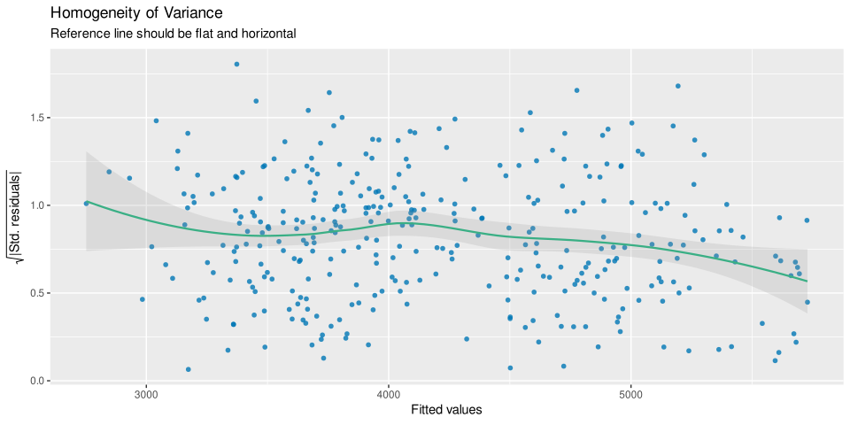
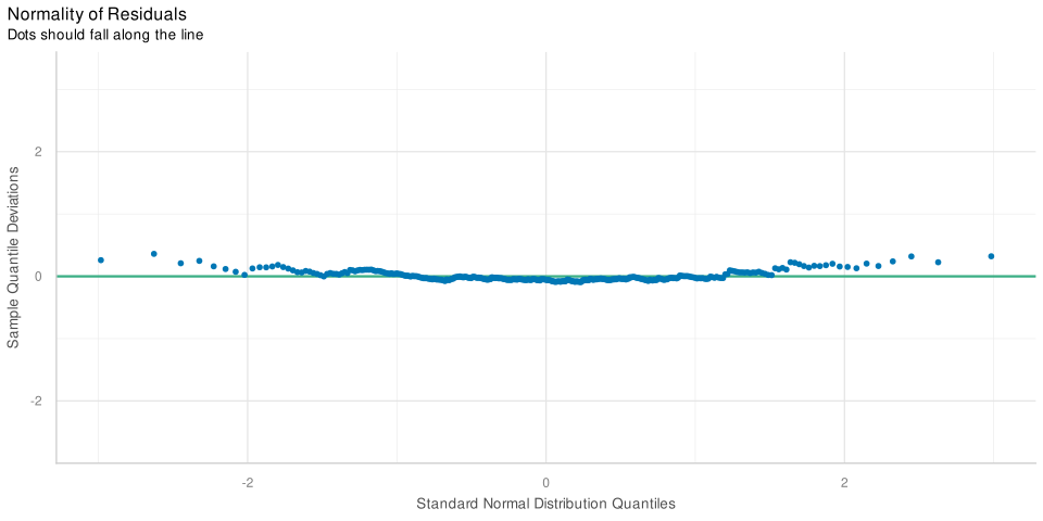
The see Package

• The see package is capable of showing a diagnostic plot appropriate for a given assumptions test

The see Package

library(palmerpenguins)
library(performance)
library(see)

# Graph for homoscedasticity
g_homo <- plot(check_heteroscedasticity(model))
# Graph for normality
g_norm <- plot(check_normality(model))

The see Package

print(g_homo)

The see Package

print(g_norm)

Robust Statistics

• A modern way of thinking about models and their assumptions is to prefer tests/models that are robust against violations of the assumptions of the general linear model

Robust Statistics

• If results from the robust models yield the same pattern of results as those from an OLS linear model, then it is unlikely the violation of assumptions ill cause an erroneous inference

• If results from the robust models show a different pattern of results than those from an OLS linear model, it signals assumptions were violated, and results from the OLS model should be suspected

• Or just use robust statistics instead of the “traditional” OLS models (see Field & Wilcox 2017)

That Was a Lot!

• I know…

• There are some ways to visually inspect a model for fit and relevant assumptions

Let’s Simplify

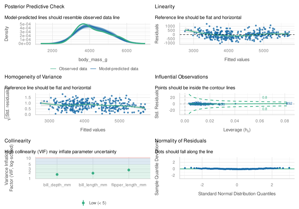
Visually Inspecting a Model

• If you run performance::check_model() you can visually inspect your model for all, or most, relevant assumptions (by looking at a single dashboard)

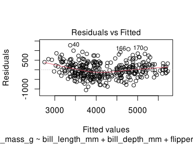
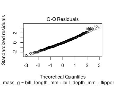
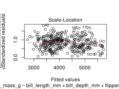
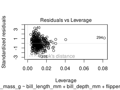
• In base R plot(model) will also show relevant graphs (one a time)

Visually Inspecting a Model

With performance:

library(performance)

check_model(model)

Visually Inspecting a Model

Visually Inspecting a Model

In base R:

plot(model)

Visually Inspecting a Model

Ways to Address Violations

• Do nothing, but report the violation/s, and that the results may be unreliable

• Transform the data to fix the violation/s (see above)

• Adjust the test statistic and/or degrees of freedom to correct for the violation/s (see above)

• Use a statistical procedure that’s robust against the violation/s (more modern approach, see above)

Ways to Address Violations

• Reporting the violation suffices (for maximum grade) for the individual assignment, but addressing it somehow will be valued (extra points) if done right

Summary of the Summary

• Look at the pretty graphs in check_model() and tell me if you see anything wrong

• Large violations of the assumptions should inspire theoretical reflection

Small N Warning

• I haven’t put much emphasis in the minimal sample size for each model

• In reality, sample size is dictated by practical constraints and should be informed by power analysis

• Still, the more variables, and the more complex model you have, the bigger your sample should be

• I don’t like rules of thumb…but Jenkins and Quintana-Ascencio 2020 found N < 8 is too small for inference, in regression, even with very little error, and N < 25 may be too small with standard conditions (regardless, power may be too low)

Small N Warning

• Estimates in small samples are less accurate than those from large samples (assuming equal variability)