| pp | pre | post | diff |
|---|---|---|---|
| pp01 | 3.155373 | 1.659283 | 1.4960897 |
| pp02 | 5.260346 | 5.163075 | 0.0972709 |
| pp03 | 0.000000 | 0.000000 | 0.0000000 |
| pp04 | 0.000000 | 0.000000 | 0.0000000 |
| pp05 | 6.098303 | 5.454262 | 0.6440405 |
| pp06 | 3.482212 | 3.150342 | 0.3318697 |
Medidas Repetidas
Desenho Experimental e Análise Avançada de Dados Ecológicos
2025-11-11
Repeated Measures Models
Dependent Samples
- So far we’ve worked with independent samples
- The observations in one group/cell are not in the other
- A penguin was either a Chinstrap, a Gentoo, or an Adelie
- A penguin was either male or female
- A penguin was either a Chinstrap male, Chinstrap female, so on and so forth
- What if I measure each unit of analysis (penguin) multiple times?
- That would be a kind of pseudo replicaton
Dependent Samples
There is a version of the tests we saw so far for dependent samples
They are trickier mathematically, but very easy in R
They can also be expressed as linear mixed models
It’s very easy to go from traditional repeated measures to mixed models in R
Questão de Partida
- Como é que eu sei se a aplicação dum tratamento/manipulação, provocou alterações numa dada variável (quantitativa)
Problema de Investigação
- Será que a aplicação dum novo tratamento reduziu o risco de conflitos/combates numa dada espécie de tubarões (o risco foi medido numa escala contínua de 0 a 10; com base nos ratings de especialistas em comportamento animal)
Delineamentos Pré vs. Pós
Um tipo de delineamento de medidas repetidas
Compara o resultado dum espécime/unidade de observação após o tratamento/manipulação com o resultado desse mesmo espécime/unidade antes do tratamento/manipulação
Delineamentos Pré vs. Pós
- Vantagens:
- Permite ter em conta a variabilidade individual/específica de cada unidade de observação
- É mais poderoso que um teste para duas amostras independentes
- Desvantagens:
- Não permite destrinçar o efeito do tratamento/manipulação do efeito da mera passagem do tempo
- É susceptível a efeitos de ordem
- Implica recolher duas vezes dados dos mesmos espécimes/unidades de observação (recolha mais longa, possibilidade de atrito/mortalidade da amostra)
Dados
Descritivas
library(dplyr) # for summarise() and group_by()
library(tidyr) # for pivot_longer() and pivot_wider()

voi <- ds[ ,c("pp", "pre", "post")]
voi <- pivot_longer(ds, -pp, names_to = "phase", values_to = "risk")

descs <- summarise(group_by(voi, phase),
                   N = n(), M = mean(risk), SD = sd(risk))

print(descs)
# A tibble: 3 × 4
phase N M SD
<chr> <int> <dbl> <dbl>
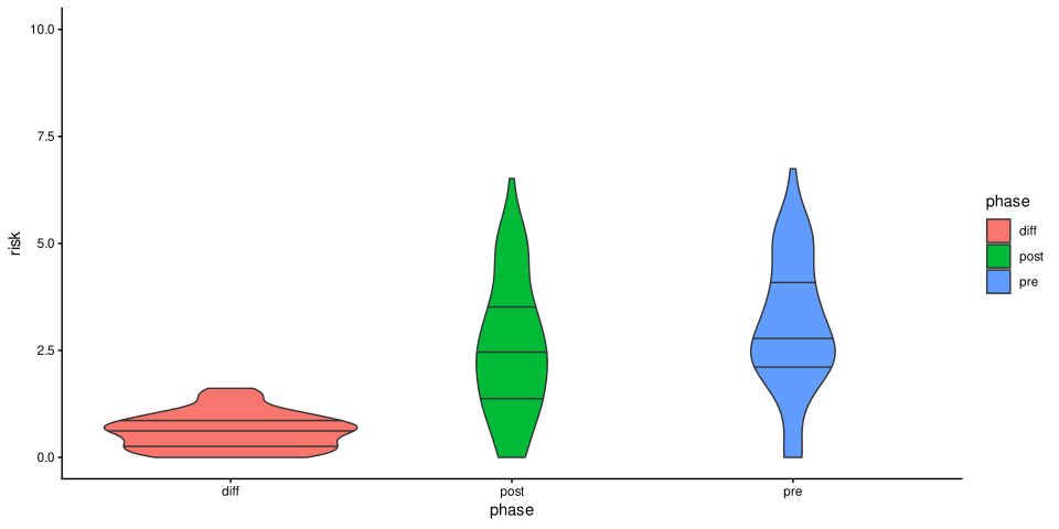
1 diff 80 0.481 0.510
2 post 80 2.56 1.57
3 pre 80 3.04 1.56 Violino
O t de Student
\(t = \frac{\bar{x}_{diff}-\mu_{diff}}{\frac{s'_{diff}}{\sqrt{N}}}; t = \frac{M_{diff} - \mu_{diff}}{SE_{diff}}\)
Graus de Liberdade
O teste trabalha a diferença entre o pré e o pós
Divide a média dessa diferença pelo erro padrão da estimação dessa média
-
Logo os graus de liberdade são os mesmos que os da média duma amostra: \(gl = N - 1\)
- O mesmo que vimos na aula anterior para o teste-t para uma amostra
Modelo com um Intercepto
Teste enquanto modelo com um intercepto ajustado às diferenças (teste-t a uma amostra aplicado às diferenças).
Call:
lm(formula = diff ~ 1, data = ds)

Residuals:
    Min      1Q  Median      3Q     Max
-1.1333 -0.3242 -0.0094  0.4303  1.4281

Coefficients:
            Estimate Std. Error t value Pr(>|t|)
(Intercept) -0.48053    0.05703  -8.427 1.28e-12 ***
---
Signif. codes:  0 '***' 0.001 '**' 0.01 '*' 0.05 '.' 0.1 ' ' 1

Residual standard error: 0.5101 on 79 degrees of freedom
H0 e H1
H0: valores dos parâmetros populacionais se a minha previsão não se verificasse (i.e., se não existir o efeito esperado na população)
H1: A negação de H0, id est, os valores possíveis para os parâmetros populacionais se o efeito estiver presente.
H0 e H1
H0: A média das diferenças entre o pré e o pós não difere do valor esperado
H1: A média das diferenças entre o pré e o pós difere do valor esperado
Pressupostos dos Testes
Os mesmos do teste-t para uma amostra
As amostras têm de ser dependentes, com todos os participantes observados nos dois momentos
Falaremos dos pressupostos mais à frente
Secção de Resultados
- Com vista a testar se o novo tratamento levava a alterações no risco de comportamentos violentos em tubarões demência, recorremos a um teste-t de student para amostras emparelhadas. Os resultados do teste indicam que há diferenças significativas entre o risco de comportamentos violentos antes e após a intervenção, sendo o risco menor após o tratamento do que antes, Mpré = 3.0438889, SD = 1.5607944, Mpós = 2.5633577, SD = 1.5743952; t(79) = 8.4265546, p < .001. Ou seja, os dados suportam a hipótese de que o tratamento é eficaz.
- Link in case it breaks
- Link in case it breaks
Early and Late Stages
Early and Late Stages
| Stage | Run | Log10Mass | Log10MR | Id | Species | |
|---|---|---|---|---|---|---|
| 173 | EARLY | Run01 | 1.263985 | -0.4351027 | ID173 | Watersipora |
| 174 | EARLY | Run01 | 1.201072 | -0.6370841 | ID174 | Watersipora |
| 175 | EARLY | Run01 | 1.146888 | -0.7427715 | ID175 | Watersipora |
| 176 | EARLY | Run01 | 1.227628 | -0.4794523 | ID176 | Watersipora |
| 177 | EARLY | Run01 | 1.256884 | -0.3818032 | ID177 | Watersipora |
| 178 | EARLY | Run01 | 1.331209 | -0.3250922 | ID178 | Watersipora |
Early and Late Stages
Let’s count the number of observations per Id.
| Id | n |
|---|---|
| ID173 | 2 |
| ID174 | 2 |
| ID175 | 2 |
| ID176 | 2 |
| ID177 | 2 |
| ID178 | 2 |
| ID179 | 2 |
| ID180 | 2 |
| ID181 | 2 |
| ID182 | 2 |
| ID183 | 2 |
| ID184 | 2 |
| ID185 | 2 |
| ID186 | 2 |
| ID187 | 2 |
| ID188 | 2 |
| ID189 | 2 |
| ID190 | 2 |
| ID191 | 2 |
| ID192 | 2 |
| ID193 | 2 |
| ID194 | 2 |
| ID195 | 2 |
| ID196 | 2 |
| ID197 | 2 |
| ID198 | 2 |
| ID199 | 2 |
| ID200 | 2 |
| ID201 | 2 |
| ID202 | 2 |
| ID203 | 2 |
| ID204 | 2 |
| ID205 | 2 |
| ID206 | 2 |
| ID207 | 2 |
| ID208 | 2 |
| ID209 | 2 |
| ID210 | 2 |
| ID211 | 2 |
| ID212 | 2 |
| ID213 | 2 |
| ID214 | 2 |
| ID215 | 2 |
| ID216 | 2 |
| ID217 | 2 |
| ID218 | 2 |
| ID219 | 2 |
| ID220 | 2 |
| ID221 | 2 |
| ID222 | 2 |
| ID223 | 2 |
| ID224 | 2 |
| ID225 | 2 |
| ID226 | 2 |
| ID227 | 2 |
| ID228 | 2 |
| ID229 | 2 |
| ID230 | 2 |
| ID372 | 2 |
| ID373 | 2 |
| ID374 | 2 |
| ID375 | 2 |
| ID376 | 2 |
| ID377 | 2 |
| ID378 | 2 |
| ID379 | 2 |
| ID380 | 2 |
| ID381 | 2 |
| ID382 | 2 |
| ID383 | 2 |
| ID384 | 2 |
| ID385 | 2 |
| ID386 | 2 |
| ID387 | 2 |
| ID388 | 2 |
| ID389 | 2 |
| ID390 | 2 |
| ID391 | 2 |
| ID392 | 2 |
| ID393 | 2 |
| ID394 | 2 |
| ID395 | 2 |
| ID396 | 2 |
| ID397 | 2 |
| ID398 | 2 |
| ID399 | 2 |
| ID400 | 2 |
| ID401 | 2 |
| ID402 | 2 |
| ID403 | 2 |
| ID404 | 2 |
| ID405 | 2 |
| ID406 | 2 |
| ID407 | 2 |
| ID408 | 2 |
| ID409 | 2 |
| ID410 | 2 |
| ID411 | 2 |
| ID412 | 2 |
| ID413 | 2 |
| ID414 | 2 |
| ID415 | 2 |
| ID416 | 2 |
| ID417 | 2 |
| ID418 | 2 |
| ID419 | 2 |
| ID420 | 2 |
| ID421 | 2 |
| ID422 | 2 |
| ID423 | 2 |
| ID424 | 2 |
| ID425 | 2 |
| ID426 | 2 |
| ID427 | 2 |
| ID428 | 2 |
| ID429 | 2 |
| ID430 | 2 |
| ID431 | 2 |
| ID432 | 2 |
| ID433 | 2 |
| ID434 | 2 |
| ID435 | 2 |
| ID436 | 2 |
| ID437 | 2 |
| ID438 | 2 |
| ID439 | 2 |
| ID440 | 2 |
| ID441 | 2 |
| ID442 | 2 |
| ID443 | 2 |
| ID444 | 2 |
| ID445 | 2 |
| ID446 | 2 |
| ID447 | 2 |
| ID448 | 2 |
| ID449 | 2 |
| ID450 | 2 |
| ID451 | 2 |
| ID452 | 2 |
| ID453 | 2 |
| ID454 | 2 |
| ID455 | 2 |
| ID456 | 2 |
| ID457 | 2 |
| ID458 | 2 |
| ID459 | 2 |
| ID460 | 2 |
| ID461 | 2 |
| ID462 | 2 |
| ID463 | 2 |
| ID464 | 2 |
| ID465 | 2 |
| ID466 | 2 |
| ID467 | 2 |
| ID468 | 2 |
| ID469 | 2 |
| ID470 | 2 |
| ID471 | 2 |
| ID472 | 2 |
| ID473 | 2 |
| ID474 | 2 |
| ID475 | 2 |
| ID476 | 2 |
| ID477 | 2 |
| ID478 | 2 |
| ID479 | 2 |
| ID480 | 2 |
| ID481 | 2 |
| ID482 | 2 |
| ID483 | 2 |
| ID484 | 2 |
| ID485 | 2 |
| ID486 | 2 |
| ID487 | 2 |
| ID488 | 2 |
| ID489 | 2 |
| ID490 | 2 |
| ID491 | 2 |
| ID492 | 2 |
| ID493 | 2 |
| ID494 | 2 |
| ID495 | 2 |
| ID496 | 2 |
| ID497 | 2 |
| ID498 | 2 |
| ID499 | 2 |
| ID500 | 2 |
| ID501 | 2 |
| ID502 | 2 |
| ID503 | 2 |
| ID504 | 2 |
| ID505 | 2 |
| ID506 | 2 |
| ID507 | 2 |
| ID508 | 2 |
| ID509 | 2 |
| ID510 | 2 |
| ID511 | 2 |
| ID512 | 2 |
| ID513 | 2 |
| ID514 | 2 |
| ID515 | 2 |
| ID516 | 2 |
| ID517 | 2 |
| ID518 | 2 |
| ID519 | 2 |
| ID520 | 2 |
| ID521 | 2 |
| ID522 | 2 |
| ID523 | 2 |
| ID524 | 2 |
| ID525 | 2 |
| ID526 | 2 |
| ID527 | 2 |
| ID528 | 2 |
| ID529 | 2 |
| ID530 | 2 |
| ID531 | 2 |
| ID532 | 2 |
| ID533 | 2 |
| ID534 | 2 |
| ID535 | 2 |
| ID536 | 2 |
| ID537 | 2 |
| ID538 | 2 |
| ID539 | 2 |
| ID540 | 2 |
| ID541 | 2 |
| ID542 | 2 |
| ID543 | 2 |
| ID544 | 2 |
| ID545 | 2 |
| ID546 | 2 |
| ID547 | 2 |
| ID548 | 2 |
| ID549 | 2 |
| ID550 | 2 |
| ID551 | 2 |
| ID552 | 2 |
| ID553 | 2 |
| ID554 | 2 |
| ID555 | 2 |
| ID556 | 2 |
| ID557 | 2 |
| ID558 | 2 |
| ID559 | 2 |
| ID560 | 2 |
| ID561 | 2 |
| ID562 | 2 |
| ID563 | 2 |
| ID564 | 2 |
| ID565 | 2 |
| ID566 | 2 |
| ID567 | 2 |
| ID568 | 2 |
Early and Late Stages
Let’s filter for n != 2
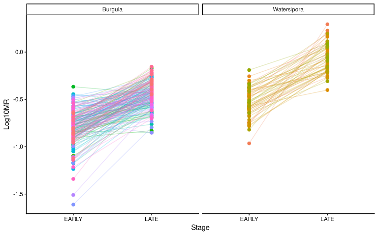
- We have exactly two observations per Id in this case
Visualisation
Visualisation
Dependence - Recap
There are different types types of dependence
Having more than one measurement per unit of observation is a case of pseudo-replication (see Hurlbert 1984; Nikinmaa et al. 2012; Bastos et al. 2013)
There are ways to statistically account for pseudo-replication
Early and Late Stages
Let’s say we want to test for differences in (log) metabolic rate (
Log10MR) per species and stage.Each unit (
Id) is from only one species (burgula or watersipora), but we have repeated measures of that unit per stage (one for early, and one for late)This is a mixed 2X2 design
Model
We’re using the
aovfunction so we can specify anErrorterm to account for individual variabilityOnly
Stageis featured in the error Term
Introducing afex
afexis a lovely R package for analyzing factorial experimentsIt automatically generates ANOVA tables with type III sums of squares, and it ensures our variables are treated as factors coded with
contr.sumIt works with
emmeansand other cool packages likeparameters,effectsize, andperformance
Introducing afex
Model
ANOVA Table
Exercise
-
Break down the effects with
emmeans- You have to be able to explain the interaction
Plot the interaction
Report the results
Complete Script v1.0
library(afex)
library(emmeans)
library(ggplot2)

options(contrasts = c("contr.sum", "contr.poly"))
afex_options(es_aov = "pes")

ds <- read.csv("../../data/bryozoan_wrangled.csv")
ds <- subset(ds, Stage != "LARVAE")
model <- aov_4(Log10MR ~ Stage * Species + (Stage | Id), ds)
emm_sp <- emmeans(model, ~ Species)
emm_st <- emmeans(model, ~ Stage)
emm_int <- data.frame(emmeans(model, ~ Species * Stage))
pc_st_sp <- pairs(emmeans(model, ~ Stage | Species))
pc_sp_st <- pairs(emmeans(model, ~ Species | Stage))
g_st_sp <- ggplot(emm_int, aes(x = Stage, y = emmean, color = Species)) +
           geom_point() + geom_errorbar(aes(ymin = lower.CL, ymax = upper.CL)) +
           geom_line(aes(group = Species)) +
           theme_classic()
g_sp_st <- ggplot(emm_int, aes(x = Species, y = emmean, color = Stage)) +
           geom_point() + geom_errorbar(aes(ymin = lower.CL, ymax = upper.CL)) +
           geom_line(aes(group = Stage)) +
           theme_classic()
Print the Results
Print the Results
Print the Results
Print the Results
Print the Results
Print the Results
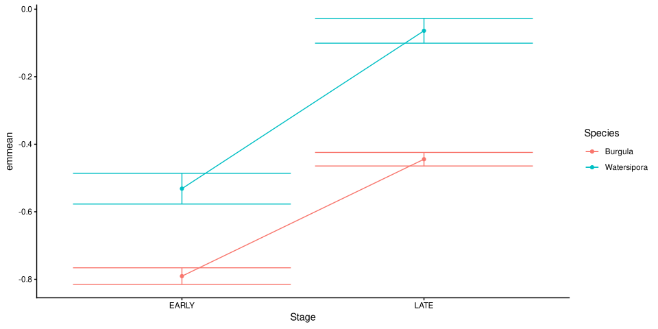
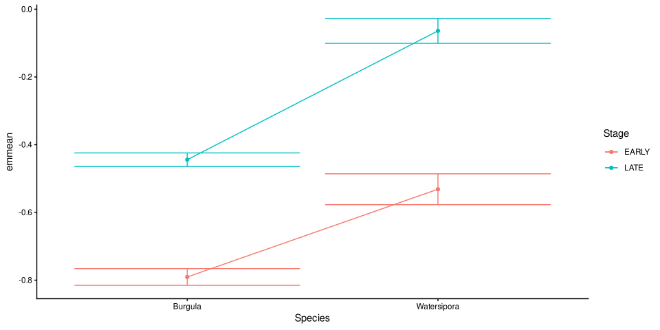
      Species Stage      emmean         SE  df   lower.CL    upper.CL
1     Burgula EARLY -0.79057356 0.01254616 253 -0.8152818 -0.76586535
2 Watersipora EARLY -0.53147617 0.02312223 253 -0.5770127 -0.48593959
3     Burgula  LATE -0.44432154 0.01015888 253 -0.4643283 -0.42431480
4 Watersipora  LATE -0.06391221 0.01872254 253 -0.1007841 -0.02704032
Understanding the Interaction
We find differences between stages (early and late) across species, and those differences are always in the same direction
We find differences between species regardless across stages, always in the same direction as well.
Thus, the interaction is likely due to the magnitude of the differences being different
Difference Between Difference
Fun Math Curiosity
We excluded larvae leaving us with a 2X2 factorial design
-
In a 2X2 design we have four cells, leaving us with a total of six possible pairs of cells:
- A - B
- A - C
- A - D
- B - C
- B - D
- C - D
Fun Math Curiosity
- Despite us having six possible pairs of cells two compare (six differences) we can only compare one difference of differences because:
- \((A - B) - (C - D) = (A - C) - (B - D) \leftrightarrow \newline A - B - C + D = A - C - B + D \leftrightarrow \newline A + (-B) + (-C) + D = A + (-C) + (-B) + D \leftrightarrow \newline A + (-B) + (-C) + D = A + (-B) + (-C) + D \leftrightarrow \newline A - B -C + D = A - B -C + D\)
Fun Math Curiosity
Hence for a 2X2 it doesn’t matter how we test for the difference between differences
 contrast                                            estimate     SE  df
 (EARLY - LATE Burgula) - (EARLY - LATE Watersipora)    0.121 0.0296 253
 t.ratio p.value
4.103 <0.0001 contrast estimate SE
(Burgula - Watersipora EARLY) - (Burgula - Watersipora LATE) 0.121 0.0296
df t.ratio p.value
253 4.103 <0.0001Understanding the Interaction
- To recap, in this 2X2 design, the interaction seems to be due to the difference between stages being larger for one species than the other
- Which is the same as saying the difference between species is larger in one stage than the other
- It’s literally the same difference (see math in previous slides)
Understanding the Main Effects
- Now that we understand the interaction, understanding the main effects is easy
Print the Results
 Species     emmean      SE  df lower.CL upper.CL
 Burgula     -0.617 0.00898 253   -0.635   -0.600
 Watersipora -0.298 0.01650 253   -0.330   -0.265

Results are averaged over the levels of: Stage
Confidence level used: 0.95 - Burgula have lower metabolic rates than Watersipora
Print the Results
 Stage emmean     SE  df lower.CL upper.CL
 EARLY -0.661 0.0132 253   -0.687   -0.635
 LATE  -0.254 0.0107 253   -0.275   -0.233

Results are averaged over the levels of: Species
Confidence level used: 0.95 - Late settlers have higher metabolic rates than early settlers
Data Wrangling I
Long to Wide
Wide to Long
Linear Mixed Models
Have I told you about linear mixed models, yet?
Like repeated measures and mixed ANOVAs they statistically account for pseudo-replication
Their math is different, and only now is the computational power required to fit them becoming mainstream
Linear Mixed Models
Linear mixed models offer some advantages over ANOVAs:
They allow for more than one error term
They forego the need to aggregate data when we have more than one observation per design cell
They work with designs that are not fully-crossed
They do not delete observations with missings in a cell
Linear Mixed Models
Linear mixed models also have their limitations:
They’re more complex than ANOVAs, taking longer to compute
There are still some open questions related to their use (e.g., best ways to estimate the degrees of freedom, best approach to model building, power analysis, etc…)
They do not fix study design limitations (and they need to be properly specified, see Arnqvist, 2020; and also Silk and collaborators (2020))
For a use case see Strien and collaborators (2012)
Linear Mixed Models
With afex linear mixed models are really easy to compute
- If we had more than one observation per stage we could have kept the model formula the same as the ANOVA
Linear Mixed Models
Looking At the Entire Dataset
| Run | Species | Stage | n |
|---|---|---|---|
| Run01 | Burgula | EARLY | 17 |
| Run01 | Burgula | LARVAE | 18 |
| Run01 | Burgula | LATE | 17 |
| Run01 | Watersipora | EARLY | 16 |
| Run01 | Watersipora | LARVAE | 20 |
| Run01 | Watersipora | LATE | 16 |
| Run02 | Burgula | EARLY | 13 |
| Run02 | Burgula | LARVAE | 32 |
| Run02 | Burgula | LATE | 13 |
| Run02 | Watersipora | EARLY | 11 |
| Run02 | Watersipora | LARVAE | 19 |
| Run02 | Watersipora | LATE | 11 |
| Run03 | Burgula | EARLY | 17 |
| Run03 | Burgula | LARVAE | 20 |
| Run03 | Burgula | LATE | 17 |
| Run03 | Watersipora | EARLY | 15 |
| Run03 | Watersipora | LARVAE | 18 |
| Run03 | Watersipora | LATE | 15 |
| Run04 | Burgula | EARLY | 19 |
| Run04 | Burgula | LARVAE | 22 |
| Run04 | Burgula | LATE | 19 |
| Run04 | Watersipora | EARLY | 16 |
| Run04 | Watersipora | LARVAE | 19 |
| Run04 | Watersipora | LATE | 16 |
| Run05 | Burgula | EARLY | 19 |
| Run05 | Burgula | LARVAE | 13 |
| Run05 | Burgula | LATE | 19 |
| Run05 | Watersipora | LARVAE | 19 |
| Run06 | Burgula | EARLY | 17 |
| Run06 | Burgula | LARVAE | 11 |
| Run06 | Burgula | LATE | 17 |
| Run06 | Watersipora | LARVAE | 20 |
| Run07 | Burgula | EARLY | 17 |
| Run07 | Burgula | LARVAE | 13 |
| Run07 | Burgula | LATE | 17 |
| Run07 | Watersipora | LARVAE | 17 |
| Run08 | Burgula | EARLY | 16 |
| Run08 | Burgula | LARVAE | 12 |
| Run08 | Burgula | LATE | 16 |
| Run08 | Watersipora | LARVAE | 20 |
| Run09 | Burgula | EARLY | 20 |
| Run09 | Burgula | LATE | 20 |
| Run09 | Watersipora | LARVAE | 20 |
| Run10 | Burgula | EARLY | 20 |
| Run10 | Burgula | LATE | 20 |
| Run11 | Burgula | EARLY | 11 |
| Run11 | Burgula | LATE | 11 |
| Run12 | Burgula | EARLY | 11 |
| Run12 | Burgula | LATE | 11 |
Looking At the Entire Dataset
All species are in all Stages and Runs
The larvae stage has fewer data suggesting we don’t have repeated measures of larvae (non fully-crossed design)
Looking At the Entire Dataset
Model
More complex model:
random slopes of: a) Species, b) Stage, and c) Species:Stage interaction, per Run
random intercepts per Run and Id
Same Pattern of Results
| Effect | df | F | p.value |
|---|---|---|---|
| Species | 1, 4.70 | 74.83 *** | <.001 |
| Stage | 2, 5.90 | 371.10 *** | <.001 |
| Species:Stage | 2, 3.36 | 63.82 ** | .002 |
We find the same main effects and interaction
Now that we have three stages we need to run pairwise comparisons to break down the effect
Rinse and Repeat
- We can revise ou script to feature this more complex model, while keeping all the other function calls
Complete Script v2.0
library(afex)
library(emmeans)
library(ggplot2)

options(contrasts = c("contr.sum", "contr.poly"))
afex_options(es_aov = "pes")

ds <- read.csv("../../data/bryozoan_wrangled.csv")
lmm <- mixed(Log10MR ~ Stage * Species + (Stage * Species | Run) + (1 | Id), ds)
emm_sp <- emmeans(lmm, ~ Species)
emm_st <- emmeans(lmm, ~ Stage)
emm_int <- data.frame(emmeans(lmm, ~ Species * Stage))
pc_st <- pairs(emm_st)
pc_st_sp <- pairs(emmeans(lmm, ~ Stage | Species))
pc_sp_st <- pairs(emmeans(lmm, ~ Species | Stage))
g_st_sp <- ggplot(emm_int, aes(x = Stage, y = emmean, color = Species)) +
           geom_point() + geom_errorbar(aes(ymin = lower.CL, ymax = upper.CL)) +
           geom_line(aes(group = Species)) +
           theme_classic()
g_sp_st <- ggplot(emm_int, aes(x = Species, y = emmean, color = Stage)) +
           geom_point() + geom_errorbar(aes(ymin = lower.CL, ymax = upper.CL)) +
           geom_line(aes(group = Stage)) +
           theme_classic()
Print the Results
Print the Results
Print the Results
Print the Results
 contrast       estimate     SE   df t.ratio p.value
 EARLY - LARVAE  -0.4911 0.0273 6.89 -17.981 <0.0001
 EARLY - LATE    -0.4376 0.0458 8.97  -9.554 <0.0001
 LARVAE - LATE    0.0535 0.0326 7.76   1.640  0.2865

Results are averaged over the levels of: Species
Degrees-of-freedom method: kenward-roger
P value adjustment: tukey method for comparing a family of 3 estimates
Print the Results
      Species  Stage      emmean         SE        df   lower.CL    upper.CL
1     Burgula  EARLY -0.79212763 0.01225351 10.705632 -0.8191882 -0.76506708
2 Watersipora  EARLY -0.55736444 0.04522981  4.438379 -0.6781989 -0.43652995
3     Burgula LARVAE -0.12831337 0.02136156  8.463025 -0.1771080 -0.07951873
4 Watersipora LARVAE -0.23897751 0.02267560  8.009655 -0.2912566 -0.18669845
5     Burgula   LATE -0.43888990 0.02251514 10.963281 -0.4884656 -0.38931416
6 Watersipora   LATE -0.03539888 0.06030172  6.448316 -0.1805005  0.10970272
Print the Results
Species = Burgula:
 contrast       estimate     SE    df t.ratio p.value
 EARLY - LARVAE   -0.664 0.0274  9.83 -24.236 <0.0001
 EARLY - LATE     -0.353 0.0285 10.97 -12.397 <0.0001
 LARVAE - LATE     0.311 0.0208  8.28  14.915 <0.0001

Species = Watersipora:
 contrast       estimate     SE    df t.ratio p.value
 EARLY - LARVAE   -0.318 0.0426  3.61  -7.466  0.0055
 EARLY - LATE     -0.522 0.0731  6.56  -7.138  0.0006
 LARVAE - LATE    -0.204 0.0601  6.43  -3.389  0.0309

Degrees-of-freedom method: kenward-roger
P value adjustment: tukey method for comparing a family of 3 estimates
Print the Results
Stage = EARLY:
 contrast              estimate     SE   df t.ratio p.value
 Burgula - Watersipora   -0.235 0.0453 4.45  -5.178  0.0049

Stage = LARVAE:
 contrast              estimate     SE   df t.ratio p.value
 Burgula - Watersipora    0.111 0.0284 8.50   3.902  0.0040

Stage = LATE:
 contrast              estimate     SE   df t.ratio p.value
 Burgula - Watersipora   -0.403 0.0529 4.04  -7.626  0.0015

Degrees-of-freedom method: kenward-roger
Print the Results
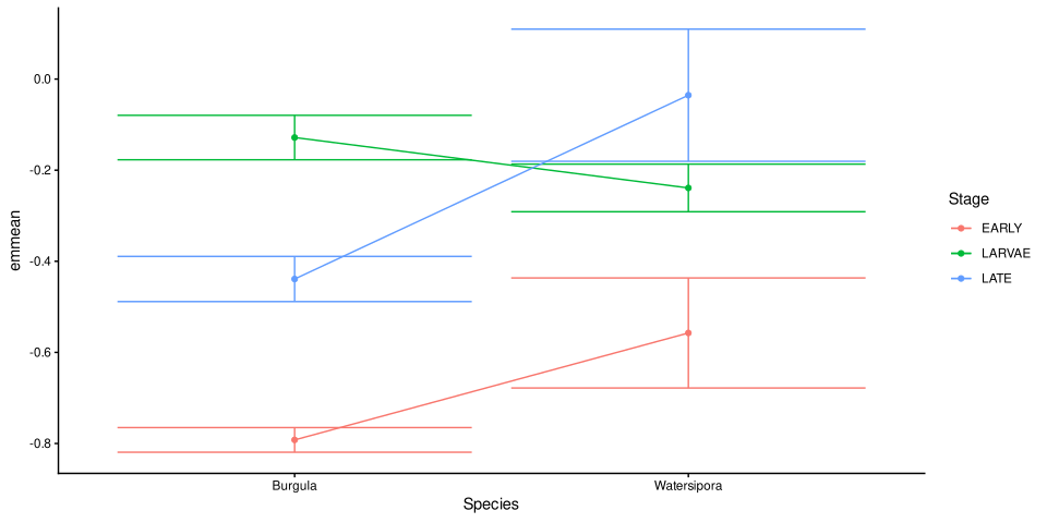
Print the Results
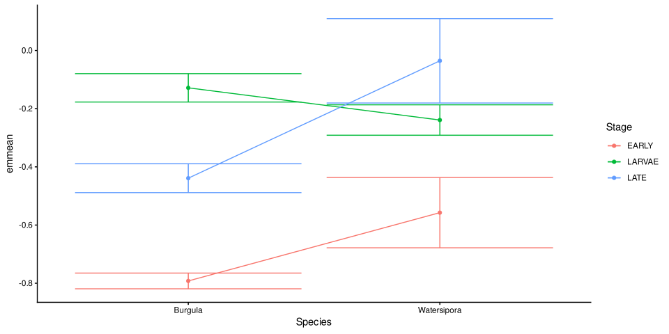
Interpretation
- How do you interpret the results?
Model Selection
There is some debate on how best to build and select linear mixed models (see Barr et al 2013; Bates et al. 2015; Singmann & Kellen 2019)
I believe a reasonable approach is to start with the maximal model warranted by the study design, and simplify until it computes without errors and/or warnings (Singmann & Kellen 2019).
Model Selection
- The maximal model warranted by the design will include random slopes and intercepts for all variables for which we have more than two repeated measures per each random effects term
Model Selection
In this case we have multiple repeated measures of “Stage” and “Species” per “Run”
Thus, will set random slopes of Stage and Species, and random intercepts per Run:
(Stage * Species | Run)
Model Selection
We have no repeated measures of Species per Id, each individual is either one species or the other
We have only two measures per Stage for some Ids, and one measure of Stage for other IDs, so we cannot add a random slope of Stage per Id
Given we have more than one measure per some Ids we can still had random intercepts per ID:
(1 | Id)
Model Selection
Thus, we arrive at our initial model:
boundary (singular) fit: see help('isSingular')Warning: lme4 reported (at least) the following warnings for 'full':
* boundary (singular) fit: see help('isSingular')Mixed Model Anova Table (Type 3 tests, S-method)
Model: Log10MR ~ Stage * Species + (Stage * Species | Run) + (1 | Id)
Data: ds
Effect df F p.value
1 Stage 2, 8.13 316.38 *** <.001
2 Species 1, 9.82 69.28 *** <.001
3 Stage:Species 2, 5.99 79.62 *** <.001
---
Signif. codes: 0 '***' 0.001 '**' 0.01 '*' 0.05 '+' 0.1 ' ' 1- It returns a warning
Model Selection
Or in a single line of code:
boundary (singular) fit: see help('isSingular')Warning: lme4 reported (at least) the following warnings for 'full':
* boundary (singular) fit: see help('isSingular')Mixed Model Anova Table (Type 3 tests, S-method)
Model: Log10MR ~ Stage * Species + (Stage * Species | Run) + (1 | Id)
Data: ds
Effect df F p.value
1 Stage 2, 8.13 316.38 *** <.001
2 Species 1, 9.82 69.28 *** <.001
3 Stage:Species 2, 5.99 79.62 *** <.001
---
Signif. codes: 0 '***' 0.001 '**' 0.01 '*' 0.05 '+' 0.1 ' ' 1- It returns a warning
Model Selection
Our model returned a warning so we’ll simplify it.
The first step in simplifhing our model will be to suppress the correlations in the random effects term:
(Stage * Species || Run)Given
Stage,Species, andRunare all categorical variables we’ll need to enableexpand_re = TRUEinmixed()to do so
Model Selection
Second model:
Mixed Model Anova Table (Type 3 tests, S-method)

Model: Log10MR ~ Stage * Species + (Stage * Species || Run) + (1 | Id)
Data: ds
         Effect       df          F p.value
1         Stage  2, 7.95 258.74 ***   <.001
2       Species 1, 13.39  84.46 ***   <.001
3 Stage:Species  2, 3.05   99.66 **    .002
---
Signif. codes: 0 '***' 0.001 '**' 0.01 '*' 0.05 '+' 0.1 ' ' 1- No warnings!
Model Selection
The second model returned no warnings, so it is our final model
It is good practice to check if the final model shows the same pattern as the initial model (Singmann & Kellen 2019)
Model Selection
| Effect | df | F | p.value |
|---|---|---|---|
| Stage | 2, 8.13 | 316.38 *** | <.001 |
| Species | 1, 9.82 | 69.28 *** | <.001 |
| Stage:Species | 2, 5.99 | 79.62 *** | <.001 |
| Effect | df | F | p.value |
|---|---|---|---|
| Stage | 2, 7.95 | 258.74 *** | <.001 |
| Species | 1, 13.39 | 84.46 *** | <.001 |
| Stage:Species | 2, 3.05 | 99.66 ** | .002 |
Model Selection
If the second model had also returned errors we would remove the random slopes for the interaction from the random effects term, then we would remove the random slopes for each variable, until we were left with only random intercepts
When the model stopped returning errors or warnings we would stop the simplification process
Model Selection
Note: If we suppress the correlations in the random effects term, remove some random slopes, and then the model computes without errors or warnings, we add back the correlations in the random effects to see if it still computes without errors, if it does we reach our final model
This gets very specific so please see Singmann 2024 for a detailed tutorial
Data Wrangling II
Import Raw Data
Separate Datasets by Species
Improve Column Names
Remove Needlesss Rows
Data Structure
The datasets are ordered thusly:
Larvae, ID01
Larvae, ID02
Larvae, ID03
Early, ID04
Early, ID05
Early, ID06
Late, ID04
Late, ID05
Late, ID06Id/Row Numbering
Id/Row Numbering
- Late settlers should have the same Ids as Early settlers, as each individual was measured twice, once at each stage
Id/Row Numbering
Prepare to bind datasets: start counting burgula sample Ids after watersipora sample Ids
Bind Datasets
Prettier Id and Run Identifiers
Save Wrangled Data
Complete Script v3.0
library(afex)
library(emmeans)
library(ggplot2)
options(contrasts = c("contr.sum", "contr.poly"))
afex_options(es_aov = "pes")
ds <- read.csv("../../data/bryozoan_raw.csv")
# Wrangle data
# Separate datasets for easier wrangling.
b <- ds[ ,1:4]
w <- ds[ ,5:8]
colnames(b) <- c("Stage", "Run", "Log10Mass", "Log10MR")
colnames(w) <- c("Stage", "Run", "Log10Mass", "Log10MR")
w <- w[w$Stage != "", ]
w$Id <- 1:nrow(w)
b$Id <- 1:nrow(b)
b$Id <- b$Id + max(w$Id)
# Late settlers should have the same Id as Early settlers
# given each bryozoan was measured twice at those stages
# Set the Ids of the late stage rows to the same as the early stage
b[b$Stage == "LATE", "Id"] <- b[b$Stage == "EARLY", "Id"]
w[w$Stage == "LATE", "Id"] <- w[w$Stage == "EARLY", "Id"]
# Start numbering burgula sample Ids after watersipora sample Ids.
b$Species <- "Burgula"
w$Species <- "Watersipora"
# Join datasets.
ds <- rbind(w, b)
# Improve random effects identifiers
ds$Id <- sprintf("ID%03d", ds$Id)
ds$Run <- sprintf("Run%02d", ds$Run)
# Model selection
lmm0 <- mixed(Log10MR ~ Stage * Species + (Stage * Species | Run) + (1 | Id), ds)
lmm1 <- mixed(Log10MR ~ Stage * Species + (Stage * Species || Run) + (1 | Id), ds,
expand_re = TRUE)
# Estimated marginal means
# Stage
emm_st <- emmeans(lmm1, ~ Stage)
# Species
emm_sp <- emmeans(lmm1, ~ Species)
# Species and Stage interaction
emm_int <- data.frame(emmeans(lmm1, ~ Species * Stage))
# Multiple comparisons
# Stage
pc_st <- pairs(emm_st)
# Stage by species
pc_st_sp <- pairs(emmeans(lmm1, ~ Stage | Species))
# Species by target
pc_sp_st <- pairs(emmeans(lmm1, ~ Species | Stage))
# Interaction plots
# Stage by species
g_st_sp <- ggplot(emm_int, aes(x = Stage, y = emmean, color = Species)) +
geom_point() + geom_errorbar(aes(ymin = lower.CL, ymax = upper.CL)) +
geom_line(aes(group = Species)) +
theme_classic()
# Species by target
g_sp_st <- ggplot(emm_int, aes(x = Species, y = emmean, color = Stage)) +
geom_point() + geom_errorbar(aes(ymin = lower.CL, ymax = upper.CL)) +
geom_line(aes(group = Stage)) +
theme_classic()