Modelos com Múltiplos Declives

Desenho Experimental e Análise Avançada de Dados Ecológicos

João O. Santos

joao.santos@ispa.pt

ISPA

2025-10-21

More than One Quantitative IV

• If we have more than one quantitative IV our proposed will have a slope for each IV

• \(Data = Model + Error; \hat{Data} = Model; Data = DV; \hat{DV} = Model\)

• \(\hat{DV} = \beta0 + \beta1 IV1 + \beta2 IV2 + \beta x IVx\)

• Link if slide breaks: https://www.kaggle.com/datasets/shreyanshverma27/water-quality-testing

Water Quality

# With a gui:
#ds <- read.csv(file.choose())
# With the file path.
ds <- read.csv("../../data/WaterQualityTesting.csv")

head(ds)

Sample.ID	pH	Temperature…C.	Turbidity..NTU.	Dissolved.Oxygen..mg.L.	Conductivity..µS.cm.
1	7.25	23.1	4.5	7.8	342
2	7.11	22.3	5.1	6.2	335
3	7.03	21.5	3.9	8.3	356
4	7.38	22.9	3.2	9.5	327
5	7.45	20.7	3.8	8.1	352
6	6.89	23.6	4.6	7.2	320

Data Tidying

# Let's rename the columns for something that's easy to work with
colnames(ds) <- c("Sample", "pH", "Temp", "NTU", "Oxygen", "Conductivity")

What Predicts Oxygen?

• What variables predict (are related) with dissolved oxygen?

Proposed Model

# All IVs
model <- lm(Oxygen ~ pH + Temp + NTU + Conductivity, ds)

Null ModelS

• It depends…

# No IV in the model
m0_0 <- lm(Oxygen ~ 1, ds)
# All IVs in the model, but no intercept
m0_1 <- lm(Oxygen ~ 0 + pH + Temp + NTU + Conductivity, ds)
# All IVs in the model but the first (pH)
m0_2 <- lm(Oxygen ~ Temp + NTU + Conductivity, ds)
# All IVs in the model but the second (Temp)
m0_3 <- lm(Oxygen ~ pH + NTU + Conductivity, ds)
# All IVs in the model but the third (NTU)
m0_4 <- lm(Oxygen ~ pH + Temp + Conductivity, ds)
# All IVs in the model but the fourth (Conductivity)
m0_5 <- lm(Oxygen ~ pH + Temp + NTU, ds)

Model Comparisons

• Test for a non-zero intercept

• When all IVs are zero is the prediction different from zero?

anova(m0_1, model)

Res.Df	RSS	Df	Sum of Sq	F	Pr(>F)
496	137.0633	NA	NA	NA	NA
495	104.8176	1	32.24569	152.2799	0

Model Comparisons

• Main effect of pH

• Is there an effect of pH when we account for the effects of all other variables?

anova(m0_2, model)

Res.Df	RSS	Df	Sum of Sq	F	Pr(>F)
496	126.8088	NA	NA	NA	NA
495	104.8176	1	21.99111	103.8528	0

Model Comparisons

• Main effect of Temp

• Is there an effect of Temp when we account for the effects of the other IVs?

anova(m0_3, model)

Res.Df	RSS	Df	Sum of Sq	F	Pr(>F)
496	104.9071	NA	NA	NA	NA
495	104.8176	1	0.0894279	0.4223222	0.516082

Model Comparisons

• Main effect of NTU

anova(m0_4, model)

Res.Df	RSS	Df	Sum of Sq	F	Pr(>F)
496	117.7840	NA	NA	NA	NA
495	104.8176	1	12.96638	61.23355	0

Model Comparisons

• Main effect of Conductivity

anova(m0_5, model)

Res.Df	RSS	Df	Sum of Sq	F	Pr(>F)
496	151.4883	NA	NA	NA	NA
495	104.8176	1	46.67063	220.4014	0

That’s Too Much Work!

Ain’t nobody got time for that meme

ANOVA Table

# We can use the `car` package to generate type III SS ANOVA tables
library(car)

Anova(model, type = 3)

	Sum Sq	Df	F value	Pr(>F)
(Intercept)	32.2456898	1	152.2798585	0.000000
pH	21.9911133	1	103.8527517	0.000000
Temp	0.0894279	1	0.4223222	0.516082
NTU	12.9663764	1	61.2335471	0.000000
Conductivity	46.6706267	1	220.4014393	0.000000
Residuals	104.8176469	495	NA	NA

• The Fs and p-values we saw before
  • Now you know that each line in an ANOVA table is a different model comparison!

Model Comparisons

Omnibus test (all or nothing)

anova(m0_0, model)

Res.Df	RSS	Df	Sum of Sq	F	Pr(>F)
499	337.4916	NA	NA	NA	NA
495	104.8176	4	232.6739	274.6999	0

• To get the F for the entire model we compare it with a model with just an intercept and no predictors

F

N <- nrow(ds)
p_m0_0 <- 1 # the intercept
p_model <- 5 # the intercept plus all IVs
SSE_m0_0 <- sum(resid(m0_0)**2)
SSE_model <- sum(resid(model)**2)
MSR <- (SSE_m0_0 - SSE_model) / (p_model - p_m0_0)
MSE <- SSE_model / (N - p_model)
F <- MSR / MSE

print(F)

[1] 274.6999

R²

• R² still gives use the ratio, or percentage (i.e., R² x 100), of the variability of the DV/outcome that our model is able to explain/predict

• \(R^2 = \frac{SSE(m0) - SSE(m1)}{SSE(m0)} = 1 - \frac{SSE(m1)}{SSE(m0)}\)

• This is a measure of effect size in a regression (more on that later)

r2 <- (SSE_m0_0 - SSE_model) / SSE_m0_0

print(r2)

[1] 0.6894214

Adjusted R²

• It is easy to get a large R² when we add multiple predictors, so we can adjust it as function of the complexity (i.e., number of parameters) of the proposed model.

• \(R_a^2 = 1 - \frac{\frac{SSE(m1)}{N - p_{m1}}}{\frac{SSE(m0)}{N - p_{m0}}} = 1 - \frac{\frac{SSE(m1)}{df_{error}}}{\frac{SSE(m0)}{df_{total}}}\)

• In multiple regressions we should report the adjusted R²_a instead of the non-adjusted one

Adjusted R²

\(R_a^2 = 1 - \frac{\frac{SSE(m1)}{df_{error}}}{\frac{SSE(m0)}{df_{total}}}\)

df_error <- N - p_model # N - 5
df_total <- N - p_m0_0 # N - 1

r2a <- 1 - ((SSE_model / df_error) / (SSE_m0_0 / df_total))

print(r2a)

[1] 0.6869117

Model Summary

summary returns the model’s F and its parameters:

• those ts are the square root of the Fs we saw before

summary(model)

Call:
lm(formula = Oxygen ~ pH + Temp + NTU + Conductivity, data = ds)

Residuals:
     Min       1Q   Median       3Q      Max 
-2.55259 -0.17601  0.03673  0.26211  1.62329 

Coefficients:
               Estimate Std. Error t value Pr(>|t|)    
(Intercept)  -19.635139   1.591156 -12.340  < 2e-16 ***
pH             2.626421   0.257724  10.191  < 2e-16 ***
Temp          -0.016087   0.024754  -0.650    0.516    
NTU           -0.417950   0.053411  -7.825 3.09e-14 ***
Conductivity   0.032833   0.002212  14.846  < 2e-16 ***
---
Signif. codes:  0 '***' 0.001 '**' 0.01 '*' 0.05 '.' 0.1 ' ' 1

Residual standard error: 0.4602 on 495 degrees of freedom
Multiple R-squared:  0.6894,    Adjusted R-squared:  0.6869 
F-statistic: 274.7 on 4 and 495 DF,  p-value: < 2.2e-16

Complete Script

# Import packages
library(ggplot2)

# Read in data
ds <- read.csv("../../data/WaterQualityTesting.csv")
# Fix colnames
colnames(ds) <- c("Sample", "pH", "Temp", "NTU", "Oxygen", "Conductivity")
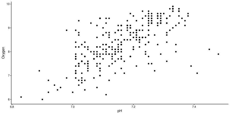
# Plot Oxygen ~ pH
pH_g <- ggplot(ds, aes(x = pH, y = Oxygen)) + geom_point() + theme_classic()
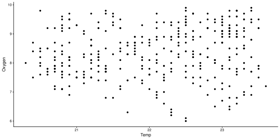
# Plot Oxygen ~ Temp
Temp_g <- ggplot(ds, aes(x = Temp, y = Oxygen)) + geom_point() + theme_classic()
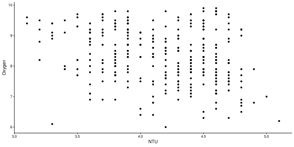
# Plot Oxygen ~ NTU
NTU_g <- ggplot(ds, aes(x = NTU, y = Oxygen)) + geom_point() + theme_classic()
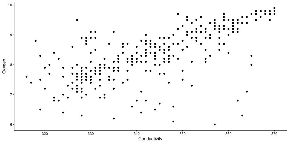
# Plot Conductivity ~ NTU
Conductivity_g <- ggplot(ds, aes(x = Conductivity, y = Oxygen)) +
                  geom_point() + theme_classic()
# Fit the Model
model <- lm(Oxygen ~ pH + Temp + NTU + Conductivity, ds)
# Hypothesis test
results <- summary(model)

Print the Results

print(pH_g)

Print the Results

print(Temp_g)

Print Results

print(NTU_g)

Print Results

print(Conductivity_g)

Print Results

print(results)

Call:
lm(formula = Oxygen ~ pH + Temp + NTU + Conductivity, data = ds)

Residuals:
     Min       1Q   Median       3Q      Max 
-2.55259 -0.17601  0.03673  0.26211  1.62329 

Coefficients:
               Estimate Std. Error t value Pr(>|t|)    
(Intercept)  -19.635139   1.591156 -12.340  < 2e-16 ***
pH             2.626421   0.257724  10.191  < 2e-16 ***
Temp          -0.016087   0.024754  -0.650    0.516    
NTU           -0.417950   0.053411  -7.825 3.09e-14 ***
Conductivity   0.032833   0.002212  14.846  < 2e-16 ***
---
Signif. codes:  0 '***' 0.001 '**' 0.01 '*' 0.05 '.' 0.1 ' ' 1

Residual standard error: 0.4602 on 495 degrees of freedom
Multiple R-squared:  0.6894,    Adjusted R-squared:  0.6869 
F-statistic: 274.7 on 4 and 495 DF,  p-value: < 2.2e-16

Exercise

• Interpret the results

• Report the results

Solutions

We have significant evidence that our model predicts the level of oxygen in the water, F_{4, 495} = 274.70, P < .001, R²_adj. = .687.

• Note: I created multiple slides so the text would fit, you don’t have to use this many paragaphs

Solutions

Results show higher pH levels are related to higher oxygen levels, β = 2.63, SE = 0.26, t₄₉₅ = 10.19, P < .001. Specifically an increase in one pH level is expected to lead to an extra 2.63mg/L of oxygen. In a similar vein, conductivity also predicts oxygen level, with each additional μS/cm increasing the estimated level of oxygen in 0.03mg/L, β = 0.03, SE < 0.01, t₄₉₅ = 14.85, P < .001.

Solutions

In turn, increases in turbidity predict decreases in oxygen level, t₄₉₅ = -7.83, P < .001. Specifically, the model predicts a decrease of 0.42mg/L of oxygen by each additional NTU, β = -0.42, SE = 0.05. Importantly, the model revealed temperature is not a significant predictor of oxygen level when we account for all other predictors (type III sums of squares), t < 1.

One Categorical IV with k > 2

• What if our categorical IV has more than two levels (k > 2)?

• With two levels (k = 2) we assigned -1 to one group and 1 to the other

• What are going to do now?

Coding Categorical Variables

• We saw there are several coding schemes

• By default R uses contr.treatement which treats one group as the baseline (i.e., 0) and compares the other groups against it

• We changed this default to contr.sum which compares groups/cells against the grand mean (the mean of all group means)

View Sum Coding

library(palmerpenguins)

# Set sum coding
options(contrasts = c("contr.sum", "contr.poly"))

ds <- penguins

# Check contrasts for a variable
contrasts(ds$species)

          [,1] [,2]
Adelie       1    0
Chinstrap    0    1
Gentoo      -1   -1

View Treatment Coding

# Set treatment coding and check contrasts for a variable
options(contrasts = c("contr.treatment", "contr.poly"))

contrasts(ds$species)

          Chinstrap Gentoo
Adelie            0      0
Chinstrap         1      0
Gentoo            0      1

More on Coding Categorical Variables

• contr.sum: Cells are compared to the grand mean. Estimates are independent of sample/cell size and interactions. Ideal for balanced factorial designs.
  • Default in SPSS, JASP, psychology
• contr.treament: Cells are compared to a reference level. Useful for unbalanced designs with no interactions and/or when a reference group exists.
  • Default in R
• For more see:
  • R Library Contrast Coding Systems for categorical variables
  • Core Guide: Dummy and Effect Coding in the Analysis of Factorial Designs

TL;DR of Coding Categorical Variables

• I’d go with contr.sum unless you have an unbalanced design (which is something to avoid if possible) and no interactions

Let’s Go with Sum Coding

# Set `contr.sum` as default coding scheme.
options(contrasts = c("contr.sum", "contr.poly"))

• Note: in this case we have no interaction and an unbalanced design, so treatment coding could arguably be a better choice

Null Model

m0 <- lm(body_mass_g ~ 1, ds)

• A model with an intercept but no predictor

• The same null model we used for the simple linear regression and the independent samples t-test

Proposed Model

model <- lm(body_mass_g ~ species, ds)

• The model with all the contrasts needed to code the categorical predictor/independent variable

• We saw that R codes the categorical predictors automatically, so the model is specified as usual

Model Comparison

# Run model comparison ANOVA
anova(m0, model)

Res.Df	RSS	Df	Sum of Sq	F	Pr(>F)
341	219307697	NA	NA	NA	NA
339	72443483	2	146864214	343.6263	0

• Write down the F and p values

Model Summary

# Get model summary
summary(model)

Call:
lm(formula = body_mass_g ~ species, data = ds)

Residuals:
     Min       1Q   Median       3Q      Max 
-1126.02  -333.09   -33.09   316.91  1223.98 

Coefficients:
            Estimate Std. Error t value Pr(>|t|)    
(Intercept)  4169.92      26.45  157.67   <2e-16 ***
species1     -469.26      34.22  -13.71   <2e-16 ***
species2     -436.83      41.80  -10.45   <2e-16 ***
---
Signif. codes:  0 '***' 0.001 '**' 0.01 '*' 0.05 '.' 0.1 ' ' 1

Residual standard error: 462.3 on 339 degrees of freedom
  (2 observations deleted due to missingness)
Multiple R-squared:  0.6697,    Adjusted R-squared:  0.6677 
F-statistic: 343.6 on 2 and 339 DF,  p-value: < 2.2e-16

Estimated Marginal Means

• The interpretation of slopes for categorical variables depends on the coding scheme and is a bit technical

• Thus, to understand and report results from models with categorical predictors we should look at the estimated marginal means for each group/cell

• If only there was a package that could help us…

  • emmeans to the rescue!!!

Estimated Marginal Means

library(emmeans)

emmeans(model, ~ species)

 species   emmean   SE  df lower.CL upper.CL
 Adelie      3701 37.6 339     3627     3775
 Chinstrap   3733 56.1 339     3623     3843
 Gentoo      5076 41.7 339     4994     5158

Confidence level used: 0.95 

Multiple Comparisons

• The one-way ANOVA is an omnibus test, it tells us if adding all the contrasts that code the IV versus not adding any significantly reduces the prediction error.
  • It is an all or nothing test
• With k > 2 there are multiple possible pairs
  • pairs = \(\frac{k (k - 1)}{2}\)
• After a significant omnibus effect we compute some multiple comparisons, either specific comparisons of interest, or all possible pairwise comparisons

Complete Script

# Import packages
library(emmeans)
library(ggplot2)
library(palmerpenguins)

# Set `contr.sum` as default categorical variable coding scheme
options(contrasts = c("contr.sum", "contr.poly"))

# Load dataset into `ds` variable
ds <- penguins
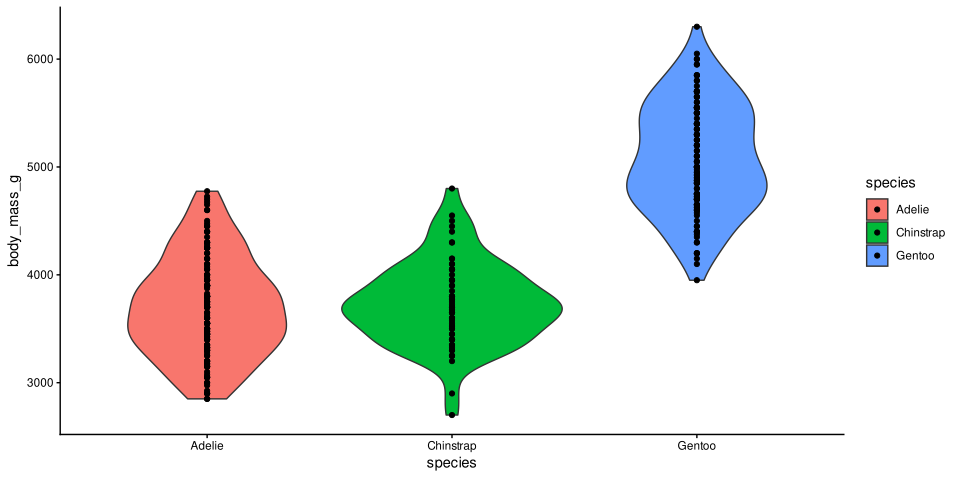
# Violin plots of mass per species with data points superimposed
graph <- ggplot(ds, aes(x = species, y = body_mass_g, fill = species)) +
         geom_violin() + geom_point() +
         theme_classic()
# Fit model
model <- lm(body_mass_g ~ species, ds)
# ANOVA table
anova_table <- anova(model)
# Estimated marginal means
emm <- emmeans(model, ~ species)
# Pairwise comparisons
pc <- pairs(emm)

Results

print(graph)

Results

print(anova_table)

Analysis of Variance Table

Response: body_mass_g
           Df    Sum Sq  Mean Sq F value    Pr(>F)    
species     2 146864214 73432107  343.63 < 2.2e-16 ***
Residuals 339  72443483   213698                      
---
Signif. codes:  0 '***' 0.001 '**' 0.01 '*' 0.05 '.' 0.1 ' ' 1

Results

print(emm)

 species   emmean   SE  df lower.CL upper.CL
 Adelie      3701 37.6 339     3627     3775
 Chinstrap   3733 56.1 339     3623     3843
 Gentoo      5076 41.7 339     4994     5158

Confidence level used: 0.95 

Results

print(pc)

 contrast           estimate   SE  df t.ratio p.value
 Adelie - Chinstrap    -32.4 67.5 339  -0.480  0.8807
 Adelie - Gentoo     -1375.4 56.1 339 -24.495 <0.0001
 Chinstrap - Gentoo  -1342.9 69.9 339 -19.224 <0.0001

P value adjustment: tukey method for comparing a family of 3 estimates 

Results

Results from a one-way ANOVA show body mass significantly differs between species, F_{2, 339} = 344.00, P < .001. Results from pairwise tests, with Tukey’s correction for multiple comparisons, show significant evidence that Gentoos are heavier (M = 5076g, SE = 41.70) than both Chinstraps (M = 3733.09g, SE = 56.06; t = 19.22, P < .001), and Adelies (M = 3700.66g, SE = 37.62; t = 24.50, P < .001). However, there is no significant evidence that Adelies and Chinstraps differ in their body mass, t < 1.