Modelos com Um Intercepto e um Declive

Desenho Experimental e Análise Avançada de Dados Ecológicos

João O. Santos

joao.santos@ispa.pt

ISPA

2025-10-14

Previously in DEAADE…

As áreas nas distribuições de probabilidades são probabilidades
- Conhecendo a distribuição e os seus parâmetros conseguimos estimar a probabilidade de obter valores num dado intervalo.
O teorema do limite central mostra-nos que a distribuição amostral da média tende para a normal, mesmo que a distribuição da população donde foram retiradas as amostras não o seja
- O desvio padrão da distribuição amostral da média é o erro padrão da média—o nosso erro de estimação

One DV and One Quantitative IV

How can we test if two variables are related?

Proposed Model

We know that the general formula is: \(Data = Model + Error\)
If two variables are related, for example, if one causes the other, then one variable is the data we’re trying to explain/predict—the dependent variable—the other variable will be the one we use to expplain/predict it—the independent variable. Hence: \(DV = \beta0 + \beta1 IV + Error\)

Proposed Model

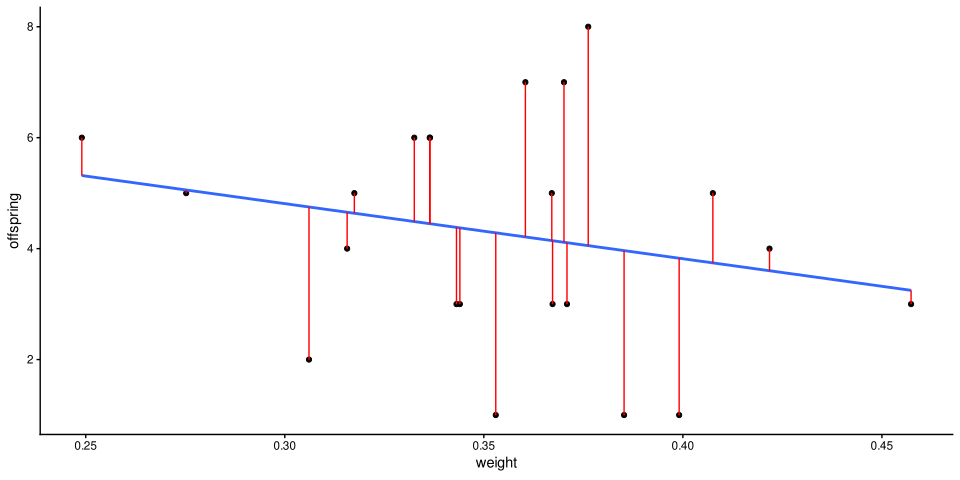
If weight predicts the number of offspring each female fish will have, then the number of offspring can be estimated as a function of the mother’s body mass

Import Data

library(readxl)

# Read excel file and store it in `ds` variable using a GUI
#ds <- read_xlsx(file.choose())
ds <- read_xlsx("../../data/weight_offspring.xlsx")

Proposed Model

If weight predicts the number of offspring each female fish will have, then the number of offspring can be estimated as a function of the mother’s body mass

# Once we import the data, which we haven't done yet, our model will be:
m1 <- lm(offspring ~ weight, ds)

Proposed Model

library(ggplot2)

ggplot(ds, aes(x = weight, y = offspring)) +
geom_point() + geom_smooth(method = "lm", se = FALSE) +
geom_errorbar(ymin = ds$offspring, ymax = predict(m1), color = "red") +
theme_classic()

Null Model

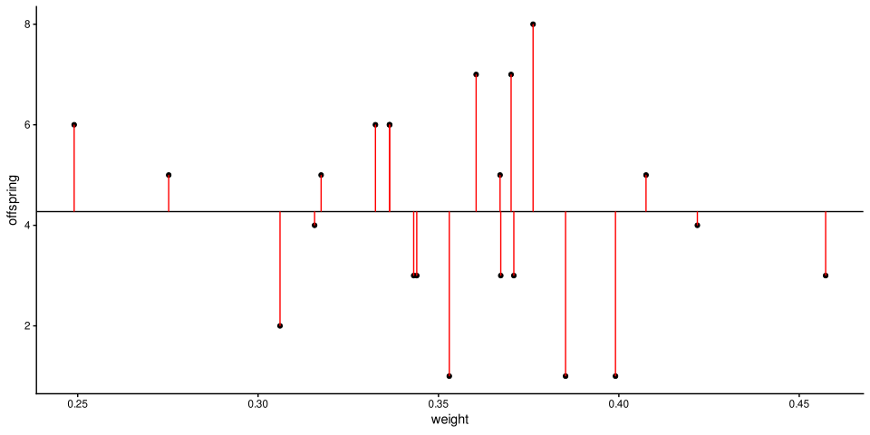
We’re going to compare our model with a simpler null model
If a mother’s weight cannot be used to predict the number of offspring she’ll have, then the number of offspring cannot be given as a function of the mother’s weight: \(DV = \beta0 + Error\)

Null Model

This model has an intercept (β0) because it wouldn’t be fair to compare a model with a slope and an intercept with a model with neither
This intercept will be the mean of the dependent variable/outcome
Note: our null model now is the proposed model from last week

Null Model

# If we had imported the data (which we haven't) the null model would be:
m0 <- lm(offspring ~ 1, ds)

# There is only one parameter, the intercept (the mean of the DV).
coef(m0)

(Intercept) 
        4.3

mean(ds$offspring)

[1] 4.3

Null Model

ggplot(ds, aes(x = weight, y = offspring)) +
geom_point() + geom_hline(yintercept = coef(m0)) +
geom_errorbar(ymin = ds$offspring, ymax = coef(m0), color = "red") +
theme_classic()

Model Comparison

anova(m0, m1)

Res.Df	RSS	Df	Sum of Sq	F	Pr(>F)
21	88	NA	NA	NA	NA
20	84	1	4.6	1.1	0.31

F

N <- nrow(ds)
p_m0 <- 1 # the intercept/beta0
p_m1 <- 2 # the intercept and a slope (beta0 and beta1)
SSE_m0 <- sum(resid(m0)**2)
SSE_m1 <- sum(resid(m1)**2)
MSR <- (SSE_m0 - SSE_m1) / (p_m1 - p_m0)
MSE <- SSE_m1 / (N - p_m1)
F <- MSR / MSE

print(F)

[1] 1.1

anova(m0, m1)

Res.Df	RSS	Df	Sum of Sq	F	Pr(>F)
21	88	NA	NA	NA	NA
20	84	1	4.6	1.1	0.31

R²

R² gives us the ratio, or percentage (i.e., R² x 100), of the variability of the DV/outcome that our model is able to explain/predict
\(R^2 = \frac{SSE(m0) - SSE(m1)}{SSE(m0)} = 1 - \frac{SSE(m1)}{SSE(m0)}\)
This is a measure of effect size in a regression (more on that later)

r2 <- (SSE_m0 - SSE_m1) / SSE_m0

print(r2)

[1] 0.052

Model Summary

The model summary shows us:

The estimate for the intercept, it’s SE, it’s t, and p-value
The estimate for the slope it’s
The F for the model comparison (the proposed vs the null model)
The R² of our model

Model Summary

model <- lm(offspring ~ weight, ds)

# The F and R2 are the ones we calculated in the previous slides
summary(model)


Call:
lm(formula = offspring ~ weight, data = ds)

Residuals:
   Min     1Q Median     3Q    Max 
-3.284 -1.316  0.153  1.448  3.946 

Coefficients:
            Estimate Std. Error t value Pr(>|t|)  
(Intercept)     7.79       3.40    2.29    0.033 *
weight         -9.94       9.52   -1.04    0.309  
---
Signif. codes:  0 '***' 0.001 '**' 0.01 '*' 0.05 '.' 0.1 ' ' 1

Residual standard error: 2 on 20 degrees of freedom
Multiple R-squared:  0.0516,    Adjusted R-squared:  0.00418 
F-statistic: 1.09 on 1 and 20 DF,  p-value: 0.309

Complete Script

library(ggplot2)
library(readxl)

# Read excel file and store it in `ds` variable using a GUI
#ds <- read_xlsx(file.choose())
# Read excel file from path and store it in `ds`.
ds <- read_xlsx("../../data/weight_offspring.xlsx")
graph <- ggplot(ds, aes(x = weight, y = offspring)) +
         geom_point() + geom_smooth(method = "lm") +
         theme_classic()
model <- lm(offspring ~ weight, ds)
results <- summary(model)

View Results

print(graph)

View Results

print(results)


Call:
lm(formula = offspring ~ weight, data = ds)

Residuals:
   Min     1Q Median     3Q    Max 
-3.284 -1.316  0.153  1.448  3.946 

Coefficients:
            Estimate Std. Error t value Pr(>|t|)  
(Intercept)     7.79       3.40    2.29    0.033 *
weight         -9.94       9.52   -1.04    0.309  
---
Signif. codes:  0 '***' 0.001 '**' 0.01 '*' 0.05 '.' 0.1 ' ' 1

Residual standard error: 2 on 20 degrees of freedom
Multiple R-squared:  0.0516,    Adjusted R-squared:  0.00418 
F-statistic: 1.09 on 1 and 20 DF,  p-value: 0.309

Report Results

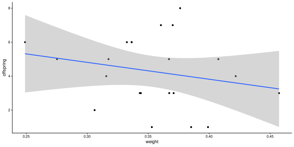
To test if the number of offspring per female are predicted by the female’s weight we fitted a simple linear regression. Results show no evidence that weight is related to the number of offspring each female fish produces, F_{1 , 20} = 1.09, P = .309, R₂ = .005.

Exercise

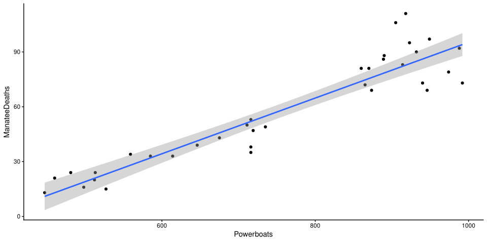
Do the number of registered power boats in a year predict the number of manatee deaths that year?

Manatees and Powerboats

Exercise 1

Import the dataset into a variable in R
Plot the data
Fit a linear regression
Print the results
Interpret the results

Solutions

library(ggplot2)

# 1.
# With a gui:
#ds <- read.csv(file.choose())
# With the file path.
ds <- read.csv("../../data/manatees.csv")

# 2.
graph <- ggplot(ds, aes(x = Powerboats, y = ManateeDeaths)) +
         geom_point() + geom_smooth(method = "lm") +
         theme_classic()

#3.
model <- lm(ManateeDeaths ~ Powerboats, ds)
# Perform model comparison/inference
results <- summary(model)

Solutions

# 4.1
print(graph)

Solutions

# 4.2
print(results)


Call:
lm(formula = ManateeDeaths ~ Powerboats, data = ds)

Residuals:
    Min      1Q  Median      3Q     Max 
-21.023  -5.645  -0.885   6.522  28.252 

Coefficients:
            Estimate Std. Error t value           Pr(>|t|)    
(Intercept) -57.1292     8.0567   -7.09 0.0000000405187601 ***
Powerboats    0.1524     0.0104   14.68 0.0000000000000005 ***
---
Signif. codes:  0 '***' 0.001 '**' 0.01 '*' 0.05 '.' 0.1 ' ' 1

Residual standard error: 11 on 33 degrees of freedom
Multiple R-squared:  0.867, Adjusted R-squared:  0.863 
F-statistic:  216 on 1 and 33 DF,  p-value: 0.0000000000000005

Solutions

There is significant evidence that the number of registered powerboats leads to an increase in the number of manatee deaths, F_{1, 33} = 215.58, P < .001, R² = .867. More specifically, it is estimated that by each 100 powerboats registered we can expect 15 additional manatee deaths that year (β = 0.152, SE = 0.01).

One DV one Dichotomic IV

What if the IV is not quantitative, but nominal with two levels
We have to find a way to “translate/code” the IV into numbers
We’ll assign -1 to one group and 1 to the other
- R will do that for us, but we have to change the defaults
- options(contrasts = c("contr.sum", "contr.poly"))

One DV one Dichotomic IV

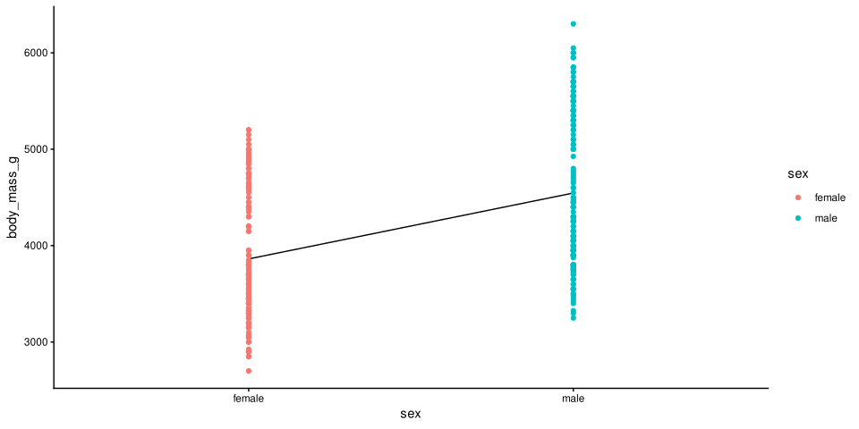
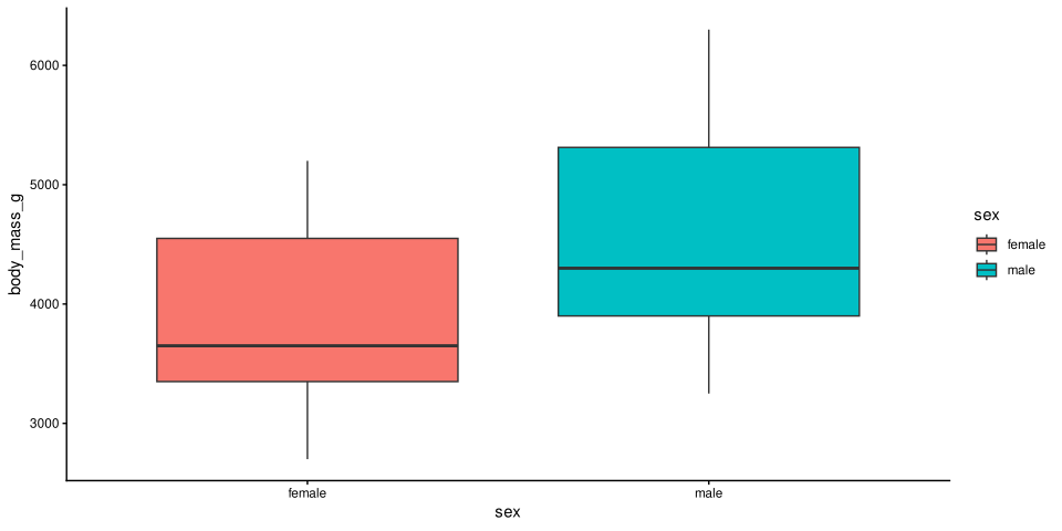
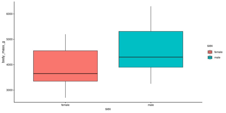
Is there a difference in the body mass between female and male penguins?

Import Data

library(palmerpenguins)

options(contrasts = c("contr.sum", "contr.poly"))

ds <- penguins

Data Tidying

# Remove penguins whose sex could not be determined
ds <- subset(ds, !is.na(sex))

Null Model

m0 <- lm(body_mass_g ~ 1, ds)

Proposed Model

m1 <- lm(body_mass_g ~ sex, ds)

Graphs

# see: https://stackoverflow.com/a/3990646
ggplot(ds, aes(x = sex, y = body_mass_g, color = sex)) +
stat_summary(fun = mean, geom = "line", group = 1, color = "black") +
geom_point() +
theme_classic()

Graphs

ggplot(ds, aes(x = sex, y = body_mass_g, fill = sex)) +
geom_boxplot() +
theme_classic()

Model Comparison

anova(m0, m1)

Res.Df	RSS	Df	Sum of Sq	F	Pr(>F)
332	215259666	NA	NA	NA	NA
331	176380769	1	38878897	73	0

Complete Script

# Import packages
library(ggplot2)
library(palmerpenguins)

# Change defaults
options(contrasts = c("contr.sum", "contr.poly"))

# Read in data
ds <- penguins
# Clean the data
ds <- subset(ds, !is.na(sex))
# Plot the data
graph <- ggplot(ds, aes(x = sex, y = body_mass_g, fill = sex)) +
         geom_boxplot() + theme_classic()
# Fit the Model
model <- lm(body_mass_g ~ sex, ds)
# Hypothesis test
results <- summary(model)

Introducing emmeans

library(emmeans)

emmeans(model, ~ sex)

 sex    emmean SE  df lower.CL upper.CL
 female   3862 57 331     3750     3974
 male     4546 56 331     4435     4656

Confidence level used: 0.95

Complete Script v2.0

# Import packages
library(emmeans)
library(ggplot2)
library(palmerpenguins)

# Change defaults
options(contrasts = c("contr.sum", "contr.poly"))

# Read in data
ds <- penguins
# Clean the data
ds <- subset(ds, !is.na(sex))
# Plot data
graph <- ggplot(ds, aes(x = sex, y = body_mass_g, fill = sex)) +
         geom_boxplot() + theme_classic()
# Fit the Model
model <- lm(body_mass_g ~ sex, ds)
# Hypothesis test
results <- summary(model)
emm <- emmeans(model, ~ sex)

Print the Results

print(graph)

Print the Results

print(results)


Call:
lm(formula = body_mass_g ~ sex, data = ds)

Residuals:
   Min     1Q Median     3Q    Max 
 -1296   -596   -237    738   1754 

Coefficients:
            Estimate Std. Error t value             Pr(>|t|)    
(Intercept)     4204         40  105.09 < 0.0000000000000002 ***
sex1            -342         40   -8.54  0.00000000000000049 ***
---
Signif. codes:  0 '***' 0.001 '**' 0.01 '*' 0.05 '.' 0.1 ' ' 1

Residual standard error: 730 on 331 degrees of freedom
Multiple R-squared:  0.181, Adjusted R-squared:  0.178 
F-statistic:   73 on 1 and 331 DF,  p-value: 0.00000000000000049

Print the Results

print(emm)

 sex    emmean SE  df lower.CL upper.CL
 female   3862 57 331     3750     3974
 male     4546 56 331     4435     4656

Confidence level used: 0.95

Running the Numbers

# Recall that we changed the default coding scheme to `contr.sum`
options(contrasts = c("contr.sum", "contr.poly"))

# Checking the contrast coding scheme for the factor.
contrasts(ds$sex)

       [,1]
female    1
male     -1

Running the Numbers

\(DV = model + Error\)

\(model = \beta0 + \beta1 \times IV\)

\(\hat{DV} = \beta0 + \beta1 \times IV\)

\(\hat{mass} = \beta0 + \beta1 \times Sex\)

Running the Numbers

\(\hat{mass_{female}} = \beta0 + \beta1 \times 1 = \beta0 + \beta1\)

\(\hat{mass_{male}} = \beta0 + \beta1 \times -1 = \beta0 - \beta1\)

Running the Numbers

\(\beta0 = \text{Grand Mean}\)

\(\beta1 = \text{Difference from each group to the Grand Mean}\)

\(\hat{mass} = \text{Grand Mean} \pm \text{difference from the GM to the group M}\)

Running the Numbers

\(\hat{mass} = 4203.98 + -341.71 \times Sex\)

\(\hat{mass_{female}} = 4203.98 + -341.71 \times 1 = 4203.98 + -341.71 = 3862.27\)

\(\hat{mass_{male}} = 4203.98 + -341.71 \times -1 = 4203.98 + 341.71 = 4545.68\)

# Same as what we get with emmeans
emmeans(model, ~ sex)

 sex    emmean SE  df lower.CL upper.CL
 female   3862 57 331     3750     3974
 male     4546 56 331     4435     4656

Confidence level used: 0.95

More than One Quantitative IV

What if we have more than one quantitative IV?
What will be our proposed model?
- Easy—the one with all the variables/predictors
What is our null model?
- It depends…
- Stay tuned for details…
When we have two or more IVs we can test for interaction effects.
- We won’t cover them today, but we will next week